Topographic effects

So far, we have largely ignored the effects of bottom topography. It was pointed out in the last chapter that bottom relief appears in the shallow water vorticity equation in the same form as the $\beta$ term and, therefore, might be expected to have similar effects. We also introduced topography as a sudden change in depth and derived edge-wave and Poincaré-wave solutions. In this chapter, we shall be more systematic and study several types of waves which rely on variable bottom topography for their existence. Perhaps more importantly, we shall consider the intimate relation between variable bottom topography and stratification.

Topographic Rossby waves

We consider first a problem which was worked out by Rhines (1970) to show the combined effects of topography and stratification. We start with the linear,

hydrostatic, Boussinesq equations $$\begin{aligned} u_t-fv & =-\frac{1}{\rho_0}p_x, \\ v_t+fu & =-\frac{1}{\rho_0}p_y, \\ 0 & =-\frac{1}{\rho_0}p_z-\frac{g\rho}{\rho_0}, \\ \rho_t+w\rho_{0z} & =0, \\ u_x+v_y+w_z & =0, \end{aligned}$$ where $\rho$ is the perturbation density and $\rho_0$ is considered constant except in the density equation. The perturbation density can be eliminated to obtain $$w=-\frac{1}{\rho_0N^2}p_{zt}$$ where $N^2=-g\rho_{0z}/\rho_0$. Expressions for the velocity can be written as $$\begin{aligned} \left(\frac{\partial^2}{\partial t^2}+f^2\right)u & =-\frac{1}{\rho_0}p_{xt}-\frac{f}{\rho_0}p_y, \\ \left(\frac{\partial^2}{\partial t^2}+f^2\right)v & =-\frac{1}{\rho_0}p_{yt}+\frac{f}{\rho_0}p_x. \end{aligned}$$ These expressions may be combined with continuity to yield $$\left[ p_{xx}+p_{yy} +\left(\frac{\partial^2}{\partial t^2}+f^2\right) \left(\frac{p_z}{N^2}\right)_z \right]_t=0.$$ If we assume time dependence of $e^{-i\sigma t}$, then this becomes $$p_{xx}+p_{yy}+(f^2-\sigma^2) \left(\frac{p_z}{N^2}\right)_z=0.$$

Now consider motions confined to a channel along the $x$ axis.

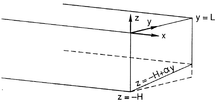
The bottom slopes gradually across the channel with bottom slope $\alpha$. The normal velocity must vanish at the sidewalls and at the bottom, while a rigid lid is assumed at the surface. The boundary conditions are $$\begin{aligned} v=0 & \quad\Rightarrow\quad i\sigma p_y+fp_x=0 & & \text{at }y=0,L, \\ w=0 & \quad\Rightarrow\quad p_z=0 & & \text{at }z=0, \\ w=\alpha v & \quad\Rightarrow\quad i\sigma(f^2-\sigma^2)p_z =\alpha N^2(i\sigma p_y+fp_x) & & \text{at }z=-H+\alpha y. \end{aligned}$$ To proceed, we scale the variables as follows: $x,y$ by $L$; $z$ by $H$; and $\omega=\sigma/f$. We also assume $N$ is constant. The problem then becomes $$\begin{aligned} p_{xx}+p_{yy}+\frac{1-\omega^2}{S^2}p_{zz} & =0, \\ i\omega p_y+p_x & =0 & & \text{at }y=0,1, \\ p_z & =0 & & \text{at }z=0, \\ i\omega(1-\omega^2)p_z & =\delta S^2(i\omega p_y+p_x) & & \text{at }z=-1+\delta y, \end{aligned}$$ where $\delta=\alpha L/H$ is the scaled bottom slope and $S=NH/fL$ is the Burger number which is a measure of the importance of stratification relative to the spatial scales of motion. The Burger number appears in virtually all cases involving both topography

and stratification. Large $S$ means strong stratification and/or large aspect ratio $H/L$ of the motion. Small $S$ means weak stratification and/or nearly horizontal motions.

For the present case, we consider low frequency motions ($\omega\ll1$) over a gently sloping bottom ($\delta\ll1$). This allows us to write the field equation and boundary conditions as $$\begin{aligned}p_{xx}+p_{yy}+\frac{1}{S^2}p_{zz}&=0,\\ p_x&=0 &&\text{at }y=0,1,\\ p_z&=0 &&\text{at }z=0,\\ i\omega p_z&=\delta S^2p_x &&\text{at }z=-1.\end{aligned}$$

The last boundary condition is appropriate because the fractional depth change across the channel is small. A solution to this problem which is freely propagating in the $x$ direction is $$p=e^{ikx}\sin(n\pi y)\cosh\mu z$$ where $\mu^2=S^2(n^2\pi^2+k^2)$ gives the vertical decay scale. Thus, strong stratification and/or short spatial scales leads to strong bottom trapping.

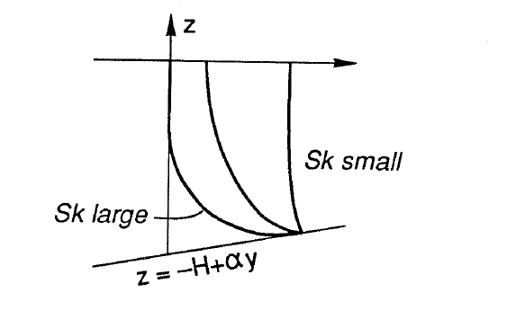
The dispersion relation is obtained by applying the bottom boundary condition $$\omega=-\frac{\delta kS^2}{\mu\tanh\mu}.$$

Notice that the waves disappear if the bottom slope vanishes $\delta\to0$ indicating the necessity of variable topography. The phase speed is always directed so that the waves move with the shallow water on their right in the northern hemisphere. So, for a bottom which shoals toward the north ($+y$), the waves propagate westward ($-x$). This is like the $\beta$-plane with nearly the same dispersion relation. If the bottom shoals toward the south ($-y$), $\delta<0$, then the waves travel eastward ($+x$). Thus, the effective north direction is the direction of shoaling.

The limit of weak stratification, $S\to0$, leads to $\mu\to0$ and $$\omega=-\frac{\delta k}{n^2\pi^2+k^2}$$ or in dimensional form $$\sigma=-\frac{\alpha kf} {H\{(n\pi/L)^2+k^2\}}.$$

This is the dispersion relation for Topographic Rossby waves, so named because of the obvious similarity to planetary Rossby waves. The vertical structure, in this case, disappears as $\mu\to0$.

Bottom-trapped waves

The waves of the previous section were indeed bottom trapped by strong stratification, but the discussion was limited to low frequencies over a gently sloping bottom. Here we relax these restrictions by considering waves along a sloping bottom in a semi-infinite fluid. The motions are still assumed to be subinertial, $\sigma<f$, but the frequency may approach $f$. This problem is also due to Rhines (1970). The field equation for pressure is $$p_{xx}+p_{yy}+\frac{f^2-\sigma^2}{N^2}p_{zz}=0$$

where $N$ is constant. The bottom is along $z=\alpha x$ where $w=\alpha u$.

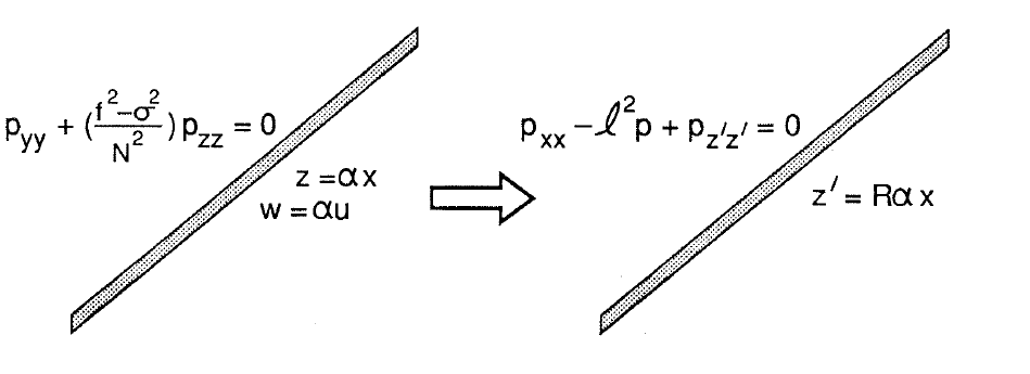
The boundary condition along the bottom is $$i\sigma(f^2-\sigma^2)p_z =\alpha N^2(i\sigma p_x-fp_y).$$ We scale $z$ by $R=N/(f^2-\sigma^2)^{1/2}$ so that $z'=zR$, and we assume a plane wave in the $y$ direction, $e^{i{ℓ} y}$. The problem becomes $$\begin{aligned} p_{xx}-{ℓ}^2p+p_{z'z'} & =0, \\ p_{z'} & =R\alpha\left(p_x-\frac{{ℓ} f}{\sigma}p\right) & & \text{at }z'=R\alpha x. \end{aligned}$$ Thus, with stratification, $R\alpha$ is the effective bottom slope. Now $$R\alpha =\frac{N\alpha}{(f^2-\sigma^2)^{1/2}} =\frac{N\alpha/f}{(1-\omega^2)^{1/2}} =\frac{S}{(1-\omega^2)^{1/2}}$$ where $S=N\alpha/f$ and $\omega=\sigma/f$. Strong stratification appears as an effectively steep bottom and vice versa. As $S\to\infty$, the bottom appears to the motions as a vertical wall. Similarly, as $\omega\to1$, the bottom appears as a vertical wall. The Burger number here can be thought of in the same way as in the last section except that $H/L$ is replaced by the bottom slope $\alpha$ because there are no distinct vertical and horizontal scales.

The angle of the bottom with respect to the horizontal is $$\theta=\tan^{-1}R\alpha.$$

This allows a solution to be written as $$p=e^{-i\sigma t+i{ℓ} y +ik(x\cos\theta+z'\sin\theta) -m(z'\cos\theta-x\sin\theta)}$$ where the time and $y$ dependences have been reinstated. In this solution, $k$ is the wavenumber parallel to the bottom, while $m$ is the wavenumber perpendicular to the bottom. The same solution could have been derived by first rotating the coordinate system to be aligned with the bottom and then rotating back. Substituting this solution into the field equation relates $k,{ℓ}$ and $m$ as $$m^2=k^2+{ℓ}^2.$$ This, along with the bottom boundary condition, yields expressions for $k$ and $m$ in terms of $\omega,{ℓ}$ and $S$, i.e. the dispersion relation; $$m=\frac{{ℓ}}{\omega} \left(\frac{S^2}{1-\omega^2+S^2}\right)^{1/2}$$

$$k=\frac{{ℓ}}{\omega} \left[ \frac{(S^2-\omega^2)(1-\omega^2)} {1-\omega^2+S^2} \right]^{1/2}.$$

Note that for decay away from the bottom ($m>0$), ${ℓ}$ and $\omega$ must have the same sign. Thus, the waves propagate only in the $+y$ direction, i.e. with shoaling water on their right just like Topographic Rossby waves. For $\omega<1$, we see that $m$ is always real, i.e. the motions are always bottom trapped. The waves propagate along the bottom ($k$ is real) as long as $\omega<S$. If $\omega>S$, then the waves decay exponentially along the bottom. This means that if $S>1$, then these waves always propagate because $\omega<1$. They become more highly bottom trapped as $S$ gets large. As $S\to0$, the waves are evanescent and less bottom trapped. As $\omega\to0$, both $k$ and $m$ become large indicating short waves trapped close to the bottom.

These properties suggest some interesting possibilities. Suppose a wave with frequency $\omega<S$ propagates along the bottom and encounters a change in bottom

slope. Without solving for the details of the solution near the corner, we know that the wave will continue to propagate as long as the new bottom slope is such that $\omega<S$. If $\omega>S$ on the new slope, then the wave must be reflected. Thus, we can imagine waves being trapped on the bottom between two gently sloping regions.

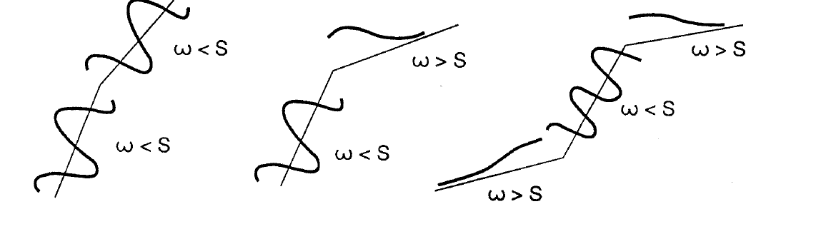
This type of behavior may occur over the continental slope between the gently sloping shelf and the gently sloping deep ocean. Of course, technically the waves would have to be sufficiently bottom trapped so that they would not feel the surface which was neglected in the problem. However, the surface should not fundamentally alter the wave behavior.

Continental shelf waves

Another type of wave motion, analogous to the topographic Rossby waves but trapped at the coast like a Kelvin wave, can occur over the continental shelf. Consider a continental shelf which borders a flat-bottom deep ocean with depth $H$. This problem was first considered by Buchwald and Adams (1968).

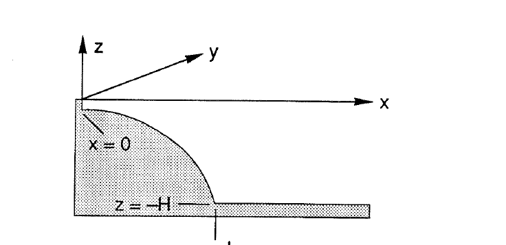
The $x$ axis points offshore while the $y$ axis is alongshore. The shelf-slope region has width $L$. We start with the shallow water equations over variable topography. We ignore stratification for now and assume that the flow is nondivergent. $$\begin{aligned} u_t-fv & =-g\eta_x, & v_t+fu & =-g\eta_y, \\ (uD)_x+(vD)_y & =0. \end{aligned}$$ The continuity equation allows us to define a transport streamfunction as $$uD=\psi_y, \qquad vD=-\psi_x.$$ Substituting into the momentum equations and eliminating the sea-surface displacement yields $$\left[ \left(\frac{1}{D}\psi_x\right)_x +\left(\frac{1}{D}\psi_y\right)_y \right]_t +f\left[ \left(\frac{1}{D}\right)_y\psi_x -\left(\frac{1}{D}\right)_x\psi_y \right]=0.$$ If the topography varies only across the shelf, i.e. $D(x)$, then this becomes $$\left(\psi_{xx}+\psi_{yy}-\frac{D_x}{D}\psi_x\right)_t +\frac{fD_x}{D}\psi_y=0.$$ We look for plane waves propagating along the shelf, $e^{-i\sigma t+i{ℓ} y}$, and assume a convenient depth profile of $$D=\begin{cases} D_0e^{2bx}, & 0<x<L, \\ D_0e^{2bL}, & x>L. \end{cases}$$

Over the shelf, the field equation reduces to $$\psi_{xx}-2b\psi_x -\left(\frac{2bf{ℓ}}{\sigma}+{ℓ}^2\right)\psi=0$$ while in the deep ocean it becomes $$\psi_{xx}-{ℓ}^2\psi=0.$$ The boundary conditions are that the velocity normal to the coast must vanish and that $\psi$ should vanish far offshore: $$u=0\quad\Rightarrow\quad\psi=0\quad\text{at }x=0,$$ $$\psi\to0\quad\text{as }x\to\infty.$$ The solution over the shelf can be written $$\psi=Ae^{b(x-L)}\sin kx.$$ Substituting this into the $\psi$ equation yields the dispersion relation $$\sigma=-\frac{2bf{ℓ}}{{ℓ}^2+k^2+b^2}$$

which looks almost identical to the Rossby wave dispersion relation showing the close correspondence of these waves to both planetary Rossby waves and topographic Rossby waves.

The solution in the deep sea is (since ${ℓ}<0$) $$\psi=Be^{{ℓ}(x-L)}.$$ The problem is closed by matching the shelf solution to the deep-sea solution. This requires that $\psi$ and $\psi_x$ be continuous at $x=L$ which leads to $$\tan kL=\frac{-k}{-{ℓ}+b}=\frac{k}{{ℓ}-b}.$$

This relation is satisfied at an infinite set of discrete values of $k$ for given ${ℓ}$ and $b$. For large $k$, the roots approach $(n+\tfrac12)\pi/L$.

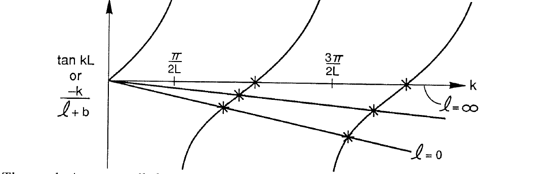
These solutions are called continental shelf waves. They are very much like planetary Rossby waves and equatorial Rossby waves. Their phases all travel with the coast on their right in the northern hemisphere. The dispersion diagram looks like

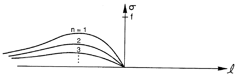
Each mode is constrained to be below some maximum frequency where $\partial\sigma/\partial{ℓ}=0$. This occurs at $$\left.{ℓ}\right|_{\sigma_{\max}}=-(k^2+b^2)^{1/2}.$$

At the maximum frequency, the group velocity is zero meaning that energy does not propagate even though phases still do. For waves that are longer than this wavelength (smaller ${ℓ}$), the wave energy propagates with the phase. For very long waves ${ℓ}\to0$, the dispersion relation becomes $$\sigma=-\frac{2bf{ℓ}}{k^2+b^2}$$ and the waves are nondispersive. This will be used to advantage later.

Waves that are shorter than those at the frequency maxima have group velocity opposite to the phase velocity. This means that the phases propagate forward through the group, but the group moves in the direction with the coast on the left in the northern hemisphere. This is essentially identical to the result for planetary Rossby waves in which phase always propagates to the west, but the group velocity may be westward or eastward depending on the wavelength of the Rossby wave. One difference is that continental shelf waves occur at discrete frequencies whereas Rossby waves form a continuum. Of course, Rossby waves would be discretized if they were constrained to a channel of some sort. The coast acts as this sort of constraint for continental shelf waves. Notice that the frequency for each mode approaches zero as the waves become very short, i.e. $\sigma\to0$ as ${ℓ}\to\infty$.

We have made a special choice for the bottom topography which made the problem rather simple by giving constant coefficients to the equation for $\psi$. It can be shown that the present results are but a special case of the results for the more general divergent equations with arbitrary cross-shelf topography. The equations are $$\begin{aligned} u_t-fv & =-g\eta_x, & v_t+fu & =-g\eta_y, \\ \eta_t+(uD)_x+(vD)_y & =0. \end{aligned}$$ If we assume that the topography does not vary along the shelf, i.e. $\partial D/\partial y=0$, and look for plane waves of the form $e^{-i\sigma t+i{ℓ} y}$, then the problem becomes $$(D\eta_x)_x-K\eta=0, \qquad K=\frac{f{ℓ}}{\sigma}D_x+{ℓ}^2D+\frac{f^2-\sigma^2}{g}.$$

The boundary conditions are $$uD=0\quad\Rightarrow\quad D\left(\eta_x-\frac{f{ℓ}}{\sigma}\eta\right)=0 \quad\text{at }x=0,$$ $$\eta\to0\quad\text{as }x\to\infty.$$

which represent no flow through the coast and coastal trapping. Huthnance (1975) has shown that, provided $D$ increases monotonically offshore, this eigenvalue problem yields an infinite discrete set of continental shelf waves which have the same general properties as those for the special case above. Further, exactly one Kelvin wave exists which can propagate at both sub- and super-inertial frequencies. Also, there is an infinite discrete set of edge waves, all at super-inertial frequencies, which can propagate in either direction. They occur outside a continuum of Poincaré waves. The complete dispersion diagram looks like

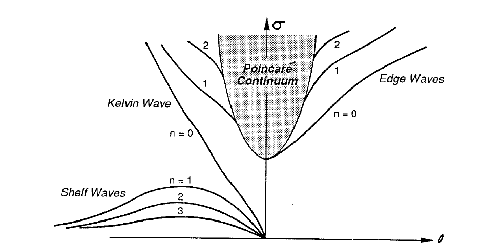
Notice the obvious similarity to the dispersion diagram for equatorial waves. In fact, most of the waves in the equatorial dispersion diagram have counterparts along the coast, except that there is no Yanai wave along a coast. Thus, to many researchers, the coastal region is essentially the same as the equator, but turned sideways. There is another important distinction, however, which we shall discuss next. That is the role of stratification. Our results from the equator were easily generalizable to a stratified ocean because the bottom was flat, so we could make use of the expansion in vertical modes and simply use a different equivalent depth to study higher modes. In contrast, waves trapped at the coast depend on the variations in topography to exist. This, along with the intimate relationship between topography and stratification which we

discussed in the previous two sections, suggests that the inclusion of stratification may not be trivial for continental shelf waves.

Coastal-trapped waves

In order to add stratification to the continental shelf wave problem, we must return to the linear, hydrostatic, Boussinesq equations with which we started the chapter. We consider a coastline oriented along the $y$ axis with $x$ pointing offshore.

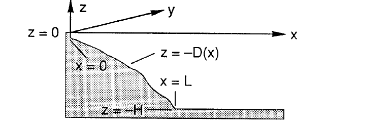
We assume that the topography varies only across the shelf and look for free waves propagating in $y$, i.e. $e^{-i\sigma t+i{ℓ} y}$. The equation and boundary conditions in terms of pressure are $$p_{xx}-{ℓ}^2p+\frac{f^2-\sigma^2}{N^2}p_{zz}=0,$$ $$(f^2-\sigma^2)p_z +N^2D_x\left(p_x-\frac{f{ℓ}}{\sigma}p\right)=0 \quad\text{at }z=-D(x),$$ $$p_z=0\quad\text{at }z=0,$$ $$p\to0\quad\text{as }x\to\infty.$$ We have taken $N$ to be constant and applied a rigid lid. However, all of the following analysis can be generalized to the case of variable $N$ and a free surface (see Huthnance, 1978).

We scale the variables as follows: $x,y$ by $L$; $z,D$ by $H$; and $\omega=\sigma/f$. The equations become $$\begin{aligned}p_{xx}-{ℓ}^2p+\frac{1-\omega^2}{S^2}p_{zz}&=0,\\ (1-\omega^2)p_z +S^2D_x\left(p_x-\frac{{ℓ}}{\omega}p\right)&=0 &&\text{at }z=-D(x),\\ p_z&=0 &&\text{at }z=0,\\ p&\to0 &&\text{as }x\to\infty,\end{aligned}$$

where $S=NH/fL$ as before. For general $D(x)$, this eigenvalue problem must be solved numerically. In fact, only a couple of special cases of $D$ are known which give analytical solutions. And these are rather unusual in their properties, so we will not study them. However, a number of important features of the free-wave solutions can be determined without solving the complete problem. These are all due to Huthnance (1978).

1. There is a singly infinite discrete set of wave modes for any choice of topography and stratification. These are called coastal-trapped waves.

2. Increased stratification, all else being equal, increases the wave frequency and makes the wave structure more horizontal.

3. The dispersion curves for all modes approach the same frequency as the wavelength decreases. This frequency is given by $$\lim_{{ℓ}\to-\infty}\omega=S\max[D_x].$$

4. The short waves (large ${ℓ}$) are identical to the bottom-trapped waves found by Rhines (1970).

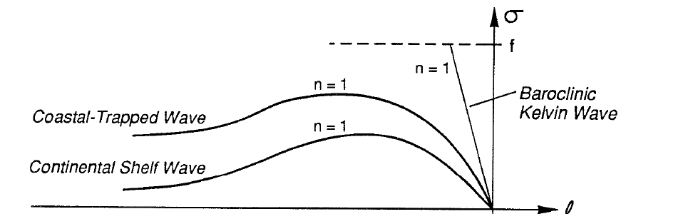
These results give the following dispersion diagram for the general case

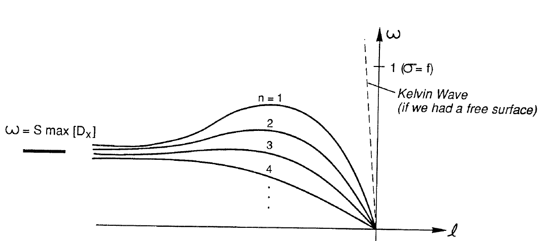
The second and third results say that the dispersion curves will go higher and higher with increasing stratification, and if $S\max[D_x]>1$ then all dispersion curves go to the inertial frequency, $\omega=1$. In dimensional form, this is $(N/f)\max[D_x]$ where $D_x$ is the actual (not scaled) bottom slope.

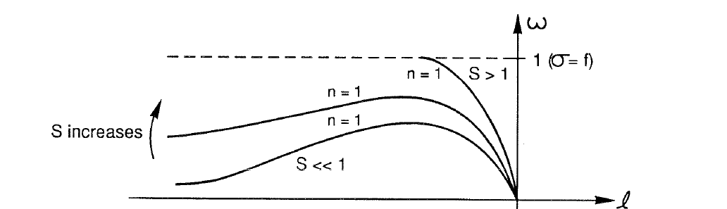
This has profound effects on the nature of the waves. They are no longer restricted to be below a maximum frequency. Now they may occur at any subinertial frequency, but they are limited in length by the wavenumber at which the dispersion curve reaches $f$. That is, each mode must be longer than a certain length to be a free wave. Consider the change that this makes on a scattering problem.

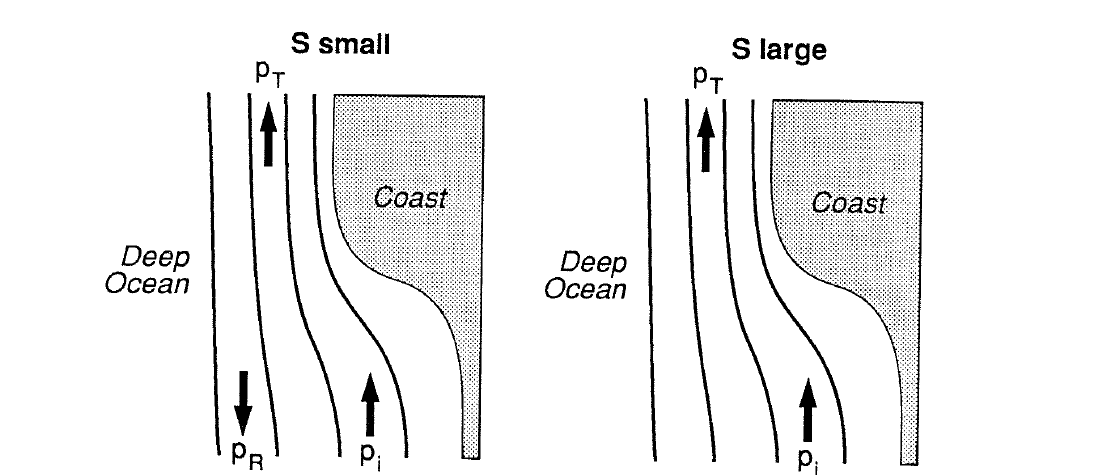
If the stratification is weak, then waves may exist which propagate energy in either direction because the group velocity changes sign. Thus, energy may be reflected as well as transmitted. If the stratification is strong so that all of the dispersion curves go to $f$, then the energy can only propagate in one direction. No energy can be reflected from the topography, no matter how tortuous the topographic variations. It turns out that in the ocean, $ND_x/f$ is often order 1, especially at low latitudes where $f$ is small. Typically, at mid-latitudes, $N/f$ is order 10 to 100, while $D_x$ is order $10^{-3}$ over the shelf but more like 0.02–0.04 over the continental slope. Remember that $N/f$ times the maximum of $D_x$ is the important value.

Before leaving this problem it is useful to consider two limiting cases.

Case A: $S\to0$. If $S$ is small, we can expand the solution in powers of $S^2$ as follows $$p(x,z)=p_0(x)+S^2p_1(x,z)+O(S^4).$$ Substituting into the full equations produces $$O(1):\qquad p_{0zz}=0$$ with $p_{0z}=0$ at both $z=0$ and $z=-D$. This means that $p_{0z}=0$ everywhere, i.e. the solution $p_0$ is vertically uniform. At the next order, we have $$O(S^2):\qquad p_{0xx}-{ℓ}^2p_0+(1-\omega^2)p_{1zz}=0.$$

$$(1-\omega^2)p_{1z} +D_x\left(p_{0x}-\frac{{ℓ}}{\omega}p_0\right)=0 \quad\text{at }z=-D,$$ $$p_{1z}=0\quad\text{at }z=0.$$ The field equation can be integrated in $z$, since $p_0$ is independent of $z$, and combined with the surface and bottom boundary conditions to yield $$(Dp_{0x})_x-\left(\frac{{ℓ}}{\omega}D_x+{ℓ}^2D\right)p_0=0$$

which is precisely the same equation that was derived for continental shelf waves, but now with a rigid lid. Thus, as we would expect, the stratified problem reduces to the barotropic problem in the limit of weak stratification.

Case B: $S\to\infty$. Based on our previous experience with stratification effects, we expect strong stratification to lead to strong bottom-trapping, i.e. short vertical scales. Basically this occurs because the stratification inhibits vertical motions. Therefore, we make a change of variables to $$\xi=x-D^{-1}(-z), \qquad \eta=Sz$$ where $D^{-1}$ is the inverse of the depth function. The new variable $\xi$ represents the horizontal distance from the bottom. The equations become, for large $S$, $$\begin{aligned} p_{\xi\xi}+(1-\omega^2)p_{\eta\eta}-{ℓ}^2p & =0, \\ D_x\left(p_\xi-\frac{{ℓ}}{\omega}p\right) & =0 & & \text{at }\xi=0, \\ p_\eta & =0 & & \text{at }\eta=0. \end{aligned}$$ A solution which satisfies the first two and the requirement that $p_z=0$ on the deep ocean bottom at $z=-1$ is $$p=e^{{ℓ}\xi/\omega} \cos\left[\frac{{ℓ}}{\omega}(\eta+S)\right].$$

Remember that ${ℓ}<0$ in the present formulation, so the solution does decay offshore. The surface boundary condition provides the dispersion relation of $$\omega=\frac{S{ℓ}}{n\pi}.$$

This is precisely the same dispersion relation as for baroclinic Kelvin waves with constant $N$.

Thus, each coastal-trapped wave mode behaves like a continental shelf wave when the stratification is weak, and then passes smoothly to a baroclinic Kelvin wave when the stratification is strong.

Consider a free wave travelling north along an eastern ocean boundary with constant $N$ and uniform $D(x)$. At low latitudes, the wave looks like a baroclinic Kelvin wave because $S$ is large. However, as the wave moves north, $S$ decreases and the wave looks more and more like a continental shelf wave. Of course, we have neglected the $\beta$ effect which would change the entire problem. So, we cannot take our thought experiment too far.

Wind-forced, long waves

We have not discussed how shelf or coastal-trapped waves might be generated. Over the past 15 years or so, a very elegant theory has evolved which suggests that the alongshelf component of the surface wind stress is an important driving mechanism.

This theory has proven quite successful in predicting shelf currents, so we will examine the basics of it. We will consider only the simplest form of the theory by Gill and Schumann (1974), but you should keep in mind that it has been generalized to a much more realistic setting.

We consider a barotropic (homogeneous) ocean as we did for the continental shelf waves.

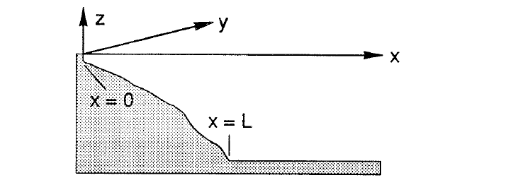
In addition, we assume that the motions occur at frequencies much less than the inertial frequency, i.e. $\sigma\ll f$, and that the alongshelf variations occur on a much larger scale than the cross-shelf motions, i.e. $\partial/\partial y\ll\partial/\partial x$. These assumptions constitute the long-wave approximation. In terms of the free-wave dispersion diagram, we are assuming that the waves are at small $\sigma$ and small ${ℓ}$. The equations of motion are $$\begin{aligned} -fv & =-g\eta_x, \\ v_t+fu & =-g\eta_y+\frac{\tau^y}{D}, \\ (uD)_x+(vD)_y & =0. \end{aligned}$$ We have also assumed a rigid lid, and imposed an alongshelf wind stress $\tau^y$. Notice that the long-wave approximation has rendered the alongshelf flow to be in geostrophic balance. This turns out to be a good approximation over most continental shelves.

We define a streamfunction as $$uD=\psi_y, \qquad vD=-\psi_x.$$

which results in an equation for $\psi$ of (with $D_y=0$) $$\left(\frac{\psi_x}{D}\right)_{xt} +\frac{fD_x}{D^2}\psi_y =\frac{D_x}{D^2}\tau^y.$$ The boundary conditions are that $\psi=0$ at $x=0$, i.e. no flow through the coast, and $\psi_x=0$ at $x=L$ which comes from matching $\psi_x$ at $x=L$. The $x$ and $y$ length scales are both order ${ℓ}^{-1}$ in the deep ocean, so $\psi_x\sim{ℓ}\psi\simeq0$ at $x=L$.

To solve this problem, we first look at free-wave solutions, i.e. $\tau^y=0$. Then we separate variables by writing $$\psi(x,y,t)=\phi(y,t)F(x).$$ The field equation becomes $$\phi_t\left(\frac{F_x}{D}\right)_x +\frac{fD_x}{D^2}\phi_yF=0$$ for which the separation works only if $$\frac{1}{c}\phi_t-\phi_y=0$$ $$\left(\frac{F_x}{D}\right)_x +\frac{fD_x}{cD^2}F=0$$

where $c$ is a separation constant. The boundary conditions become $F=0$ at $x=0$ and $F_x=0$ at $x=L$.

The problem for $F$ is a Sturm–Liouville eigenvalue problem and it can be shown that the eigenfunctions, $F_n$, satisfy the orthogonality relation $$\int_0^L\frac{D_x}{D^2}F_nF_m\,dx=\delta_{nm}$$

where $\delta_{nm}$ is the Kronecker delta. Each $F_n$ corresponds to the cross-shelf structure of a free-wave mode. The problem for $\phi$ is just a first-order wave equation with the solution $$\phi=\phi_0(y+ct).$$

where $\phi_0$ is any function. Thus, we see that each wave mode need not be sinusoidal in shape and that the eigenvalue $c$ is simply the phase speed of the free wave. The waves move in the $-y$ direction as expected and they are nondispersive (as shown for the small ${ℓ}$ limit of the continental shelf wave problem).

These results allow the forced problem to be solved by expanding $\psi$ in the set of free-wave modes $$\psi(x,y,t)=\sum_n\phi_n(y,t)F_n(x).$$ Substituting this into the field equation and using the orthogonality condition of the free modes yields $$\frac{1}{c_n}\phi_{nt}-\phi_{ny}=-b_n\tau^y$$

where $$b_n=\frac{1}{f}\int_0^L\frac{D_x}{D^2}F_n\,dx$$ are the wind-coupling coefficients which tell how well the wind stress drives each mode. The solution to this equation is $$\phi_n(y,t) =\phi_n\left(0,t+\frac{y}{c_n}\right) +b_n\int_0^y \tau^y\left(\xi,t+\frac{y-\xi}{c_n}\right)d\xi.$$ This solution simply says that $\phi(y,t)$ is given by the $\phi$ that propagated into the domain at the origin of integration plus the integrated effect of the wind generating free waves along the coast. Thus, the entire wind-forced problem has boiled down to a rather simple integral of the wind stress displaced in time by the period needed for the free wave to propagate from its generation location $\xi$ to the prediction site $y$.

The overall solution procedure is as follows. The free-wave phase speeds and cross-shelf structures are computed from the eigenvalue problem. These are used to compute the $b_n$. Then the first-order wave equation is integrated for each mode and

the streamfunction is reconstructed as the appropriate summation of modes. Crucial to this approach is the long-wave approximation which renders the waves nondispersive allowing the separation of variables. This approach does not work for dispersive waves. This theory has been extended to a remarkable degree of sophistication in which alongshelf variations in stratification, bottom topography and bottom friction have been incorporated.