Chapter 1
Basic concepts
Waves are not easy to define. Whitham (1974) defines a wave as “a recognizable signal that is transferred from one part of a medium to another with recognizable velocity of propagation”. This is a very broad definition and encompasses an enormous range of dynamical systems as well as physical processes. That is, waves can occur in many different media and take on many different forms. We often think of waves as simple sinusoidal undulations of some substance, but this view is too restricted and often not very useful.
In this course, we will consider a number of different types of waves and wave motions in the ocean and in the atmosphere. They will be found to occur at many different time and space scales. In general, wave-like fluctuations of flow fields are not exact solutions of the continuum formulation of momentum and mass conservation and the laws of thermodynamics. However, they often represent good approximate solutions of those equations.
Therefore, the first step in discussing wave motion is the appropriate simplification of the field equations to obtain a set whose solutions are waves. In most of what we do, this involves linearizing the field equations about some basic state of rest or of quasi-steady motion. That is, products of any dependent variables in the equations are typically assumed to be small in relation to the other terms. It usually proves possible, by this device, to obtain waves as solutions of the linearized equations.
Because the equations are linear, we are entitled to superpose solutions of the equations in order to find solutions to more general initial and boundary value problems. This is one of the real beauties of linear wave theory. We will spend most of our time studying such linear waves and their properties before relaxing the linearization condition which precludes nonlinear interactions.
As we will see, there are many different waves with quite different characteristics which can exist within the framework of rotating fluid systems such as the ocean and the atmosphere. In order to proceed, certain concepts and approaches which are common to most studies of linear waves should be understood first. Some of these are presented next.
Plane waves
The basic state of rest or quasi-steady flow about which the waves are linear perturbations defines the medium through which the waves propagate. If we assume that the medium is homogeneous in space and time (even if it strictly is not), then possible solutions often have the form of a plane wave: \[\phi(\vec{x},t)=\Re\,A e^{i(\vec{k}\cdot\vec{x}-\sigma t)}.\]
where \(\phi(\vec{x},t)\) are the dependent variables (i.e., velocity \(\vec{u}\), pressure \(p\), density \(\rho\), etc.), \(A\) is the amplitude, \(\vec{k}=(k,\ell,m)\) is the wavenumber, \(\sigma\) is the radian frequency, and \(\Re\) means that we take the real part of the expression. Customary auxiliary definitions are \[\lambda=2\pi/|\vec{k}|=\text{wavelength},\qquad f=\sigma/2\pi=\text{frequency},\qquad T=2\pi/\sigma=1/f=\text{period}.\]
Since \(A\) is complex, it carries with it not only amplitude but also phase information. We could, of course, write \[\phi(\vec{x},t)=|A|\cos\left(\vec{k}\cdot\vec{x}-\sigma t +\tan^{-1}\frac{\Im A}{\Re A}\right)\] where \(\Im\) refers to the imaginary part of the expression. However, it is often much more convenient to work with the complex form of all variables and to take the real parts only at the very end. This is always possible because we have linearized the field equations.
The convention \(e^{i(\vec{k}\cdot\vec{x}-\sigma t)}\) is preferable to the convention \(e^{i(\vec{k}\cdot\vec{x}+\sigma t)}\) because, in the first case, wave ‘crests and troughs’ move in the direction of \(\vec{k}\) when \(\sigma>0\). This can be seen by examining the phase of the wave, namely \(\vec{k}\cdot\vec{x}-\sigma t\). Surfaces of constant phase, \(\vec{k}\cdot\vec{x}-\sigma t=\Phi_0\), are planes normal to \(\vec{k}\) and moving outward along \(\vec{k}\) as \(t\) increases (for \(\sigma>0\)). In two dimensions we have
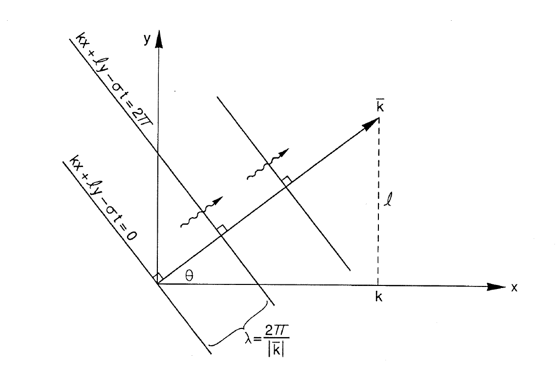
The speed at which phase planes move along \(\vec{k}\) is the phase speed \[c=\sigma/|\vec{k}|=\lambda/T.\] It is directed along \(\vec{k}\). Note that the speed of phase plane intersection with the \(x\)-axis is not \(c\cos\theta\) but rather is \[\frac{c}{\cos\theta} =\left(\frac{\sigma}{|\vec{k}|}\right) \left(\frac{|\vec{k}|}{k}\right) =\sigma/k\] which can be considerably faster than \(c\). In fact, as \(\theta\to\pi/2\), the phase speed in the \(x\)-direction approaches infinity!
The form \(Ae^{i(\vec{k}\cdot\vec{x}-\sigma t)}\) is called a ‘travelling plane wave’. The superposition of oppositely travelling plane waves \[Ae^{i(\vec{k}\cdot\vec{x}-\sigma t)} +Ae^{i(-\vec{k}\cdot\vec{x}-\sigma t)} =2Ae^{-i\sigma t}\cos(\vec{k}\cdot\vec{x})\] is called a standing wave because the crests and troughs do not propagate with time. It is not always possible to construct such a superposition because oppositely travelling plane waves are not always possible and, even when possible, may have different wavenumbers.
The dispersion relation
All of the foregoing is kinematics, true for any given \(\sigma,\vec{k}\) with no physics. The physics are contained in the dispersion relation \[\sigma=\Omega(\vec{k})\] which is obtained by requiring the plane waves to be solutions of the linearized, dissipationless equations of motion. The following table contains some examples of wave equations (all of which we will encounter later) with their respective dispersion relations.
| Linearized Equation | Plane wave | Dispersion Relation | |
| a) | \(\phi_t+c_0\phi_x=0\) | \(e^{ikx-i\sigma t}\) | \(\sigma=c_0k\) |
| b) | \(\phi_{tt}-c_0^2\phi_{xx}=0\) | \(e^{ikx-i\sigma t}\) | \(\sigma^2=c_0^2k^2\) |
| c) | \(\phi_t+\vec c_0\cdot\nabla\phi=0\) | \(e^{i\vec{k}\cdot\vec{x}-i\sigma t}\) | \(\sigma=\vec c_0\cdot\vec{k}\) |
| d) | \(\phi_{tt}-c_0^2\nabla^2\phi=0\) | \(e^{i\vec{k}\cdot\vec{x}-i\sigma t}\) | \(\sigma^2=c_0^2|\vec{k}|^2\) |
| e) | \(\nabla^2\phi_t+\beta\phi_x=0\) | \(e^{i\vec{k}\cdot\vec{x}-i\sigma t}\) | \(\sigma=-\beta k/|\vec{k}|^2\) |
Each linearized equation is a statement of approximate dynamical and thermodynamical conservation laws. All are solved using plane waves of the type discussed above. All require different dispersion relations, and the solutions have different properties. For cases (a)–(d), the phase speed \(c=\sigma/|\vec{k}|\) is independent of wavelength, frequency or direction. Such waves are nondispersive or dispersionless because all waves (for each case individually) travel with the same speed. In case (e), the phase speed \(c\) is dependent upon the wavelength and the direction, so these waves are dispersive. As we will see, this basically means that a group of such
waves will not remain together while propagating through the medium, but instead will break up or disperse. Standing waves, as defined above, are possible in cases (b) and (d) because oppositely travelling waves can occur with the same wavenumber but with frequencies of opposite sign. That is, the dispersion relation has more than one branch, \(\sigma=\Omega_j(\vec{k})\) for \(j=1,\ldots,n\). However, in cases (a), (c) and (e), a given wavenumber corresponds to only a single frequency (only one branch), i.e. waves can travel only in one direction, so standing waves are not possible.
Several cautionary notes are in order here. Plane waves are rarely the complete solution to any boundary or initial value problem. If the medium is actually homogeneous and steady, then plane waves may often be superposed to solve such problems. However, often the medium is not homogeneous or steady, so plane wave solutions then require modifications before they can be used. We shall spend a good part of this course deriving linearized equations which isolate particular physics and we shall discuss the appropriate plane wave solutions in detail. But it must be kept in mind that, in order to establish a basis for comparison with observations of real systems, a boundary or initial value problem must be solved, most probably including medium inhomogeneities. We shall, in some instances, show examples of such problems for some sets of linearized equations.
Linear superposition of plane waves
In a homogeneous medium, initial value problems are solvable as Fourier integrals which amounts to summing an infinite number of plane wave solutions. If the dispersion relation has \(n\) branches \[\sigma=\Omega_j(\vec{k}),\qquad j=1,\ldots,n\]
then \(n\) initial conditions are normally required. The solution takes the form \[\phi(\vec{x},t)=\sum_{j=1}^n \iiint_{-\infty}^{\infty} A_j(\vec{k})e^{i[\vec{k}\cdot\vec{x}-\Omega_j(\vec{k})t]} \,d\vec{k}\] where the \(A_j(\vec{k})\) are fixed by the initial conditions. For example, if \(n=1\), and we are in one dimension \[\sigma=\Omega(k)\] \[\phi(x,t)=\int_{-\infty}^{\infty} A(k)e^{i[kx-\Omega(k)t]} \,dk.\] \(A(k)\) is fixed by specifying \(\phi(x,0)\), that is \[\phi(x,0)=\int_{-\infty}^{\infty}A(k)e^{ikx}\,dk; \qquad A(k)=\frac{1}{2\pi}\int_{-\infty}^{\infty}\phi(x,0)e^{-ikx}\,dx.\] Notice that if \(\Omega=ck\), then \[\phi(x,t)=\int_{-\infty}^{\infty}A(k)e^{ik(x-ct)}\,dk =\int_{-\infty}^{\infty}A(k)e^{ikx'}\,dk =\phi(x-ct,0).\] This means that, in this special case, the initial condition \(\phi(x,0)\) translates towards \(x>0\) at speed \(c\) without changing shape.
For homogeneous media, therefore, the problem is generally solved by (i) finding the dispersion relation, (ii) deducing the \(A_j(\vec{k})\) from initial conditions, and (iii) evaluating a set of Fourier integrals.
The method of stationary phase: Group velocity
The greatest difficulty with the above procedure is most often that the integrals are hard to do. A very useful approximate technique with physical content is the method
of stationary phase. As a preview, let us consider a one-dimensional example with the special initial condition \(\phi(x,0)=a(x)e^{ik_0x}\).
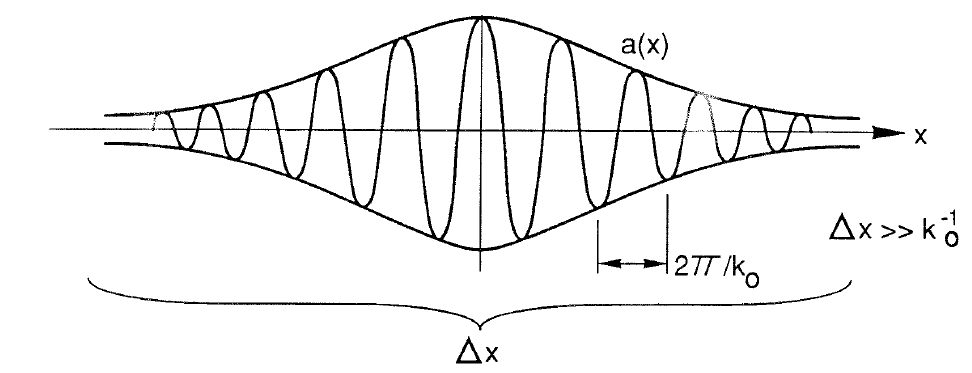
This represents a slowly modulated plane wave with envelope \(a(x)\). We can always write \[\phi(x,0)=\int_{-\infty}^{\infty}A(k)e^{ikx}\,dk; \qquad A(k)=\frac{1}{2\pi}\int_{-\infty}^{\infty}\phi(x,0)e^{-ikx}\,dx\] and so \[A(k)=\frac{1}{2\pi}\int_{-\infty}^{\infty} a(x)e^{i(k_0-k)x}\,dx; \qquad a(x)=\int_{-\infty}^{\infty}A(k)e^{i(k-k_0)x}\,dk.\] In the integral for \(A(k)\), the contribution to the integral itself is mostly from the regions where the quantity \((k_0-k)x\) is small. In fact, where this quantity is large, \(e^{i(k_0-k)x}\) oscillates rapidly and the integrated parts cancel each other. Moreover, \(a(x)=0\) for \(x\gg\Delta x\). So, \(A(k)\) is centered around \(k_0\) and peaked there for this special choice of \(\phi(x,0)\).
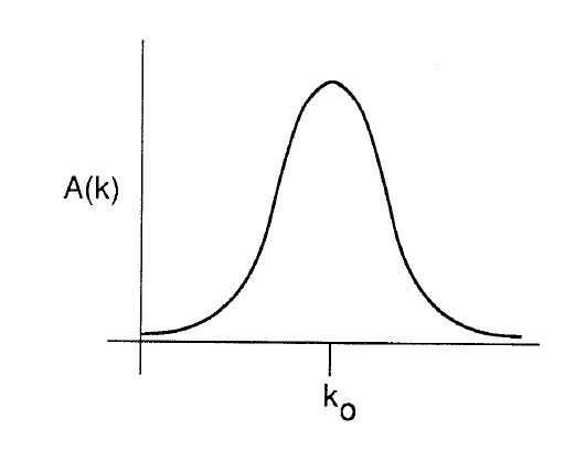
The modulated plane wave is said to be a ‘narrow band signal’.
We can evaluate \(\phi(x,t)\) by expanding \(\Omega(k)\) in a Taylor series about \(k_0\): \[\begin{aligned} \phi(x,t) & =\int_{-\infty}^{\infty}A(k)e^{i[kx-\Omega(k)t]}\,dk \\ & \simeq\int_{-\infty}^{\infty}A(k) e^{i[kx-\Omega(k_0)t-(k-k_0)(\partial\Omega/\partial k)|_{k=k_0}t]}\,dk \\ & =\int_{-\infty}^{\infty}A(k) e^{i[kx-\Omega(k_0)t-(k-k_0)(\partial\Omega/\partial k)|_{k=k_0}t]} e^{ik_0x-ik_0x}\,dk \\ & =e^{i[k_0x-\Omega(k_0)t]} \int_{-\infty}^{\infty}A(k) e^{i(k-k_0)[x-(\partial\Omega/\partial k)|_{k=k_0}t]}\,dk. \end{aligned}\] That is \[\phi(x,t)=e^{i[k_0x-\Omega(k_0)t]} a\left(x-\left.\frac{\partial\Omega}{\partial k}\right|_{k=k_0}t\right).\] The modulating envelope moves at a velocity \(\left.\partial\Omega/\partial k\right|_{k=k_0}\), defined by the dispersion relation \(\sigma=\Omega(k)\). This velocity is called the group velocity \[c_g=\left.\frac{\partial\Omega}{\partial k}\right|_{k=k_0}\] and is not, in general, equal to the phase speed \(c=\sigma/k\) of the modulated plane wave. Therefore, the dominant wavelength \(\lambda=2\pi/k_0\) has two speeds associated with it. They are the phase speed \(c=\sigma/k_0=\Omega(k_0)/k_0\) and the group velocity \(c_g=\partial\sigma/\partial k|_{k=k_0}=\partial\Omega/\partial k|_{k=k_0}\). The modulated envelope thus moves through the phases of the underlying plane wave rather than with them.
The restriction to narrow band processes is illustrative but not necessary. Consider \[\phi(x,t)=\int_{-\infty}^{\infty}A(k)e^{i[kx-\Omega(k)t]}\,dk.\] Define \[\Theta(k;x,t)=kx/t-\Omega(k).\] Then \[\phi(x,t)=\int_{-\infty}^{\infty}A(k)e^{it\Theta(k;x,t)}\,dk.\]
The Riemann–Lebesgue theorem (e.g. Bender and Orszag, 1978, pp. 277–278) says that if \(\int_{-\infty}^{\infty}A(k)\,dk\) exists, then \(\lim_{t\to\infty}\int_{-\infty}^{\infty}A(k)e^{itk}\,dk=0\). Hence, we get little contribution to \(\phi(x,t)\) unless \(\Theta(k;x,t)\) has no variation with \(k\), i.e., unless there exist \(k_0\) such that \(\left.(\partial\Theta/\partial k)\right|_{k_0}=0\). Perhaps a more intuitive statement is that the integrand looks like

in which the rapid oscillations of \(e^{it\Theta}\), as \(t\to\infty\), cancel unless \(\partial\Theta/\partial k=0\) somewhere.
Stationary phase now asserts \[\phi(x,t)\simeq\int_{-\infty}^{\infty}A(k) e^{it[\Theta(k_0)+(k-k_0)\Theta'(k_0) +(k-k_0)^2\Theta''(k_0)/2]}\,dk.\] In other words, at a given \(x\) and \(t\), the greatest contribution to \(\phi(x,t)\) is from that wavenumber \(k_0\) at which \(\Theta'(k_0;x,t)=0\). Since \(\Theta(k;x,t)=kx/t-\Omega(k)\) we have \[x/t-\left.\frac{\partial\Omega}{\partial k}\right|_{k_0}=0\] which means that the wavenumber \(k_0\) that makes the biggest contribution to \(\phi(x,t)\) is the one for which \[\left.\frac{\partial\Omega}{\partial k}\right|_{k_0}=x/t;\] i.e., the one whose group velocity is \(x/t\).
To estimate that contribution, realise that \(\Theta'(k_0)=0\), so that \[\phi(x,t)\simeq A(k_0)e^{it\Theta(k_0)} \int_{-\infty}^{\infty} e^{i(k-k_0)^2\Theta''(k_0)t/2}\,dk.\]
or, since \(\int_{-\infty}^{\infty}e^{-\alpha x^2}\,dx=(\pi/\alpha)^{1/2}\), then \[\phi(x,t)\simeq A(k_0)e^{it\Theta(k_0)} [2\pi/-it\Theta''(k_0;x,t)]^{1/2}\] \[\phi(x,t)\simeq A(k_0)e^{i[k_0x-\Omega(k_0)t]} [2\pi/-it\Theta''(k_0;x,t)]^{1/2}.\] The solution is thus a slowly modulated plane wave whose wavenumber \(k_0\) is characterized by \[\left.\frac{\partial\Omega}{\partial k}\right|_{k_0}=x/t.\]
The solution is only valid for very large \(t\) and \(x\) because it requires the rapid oscillation of \(e^{i[kx-\Omega(k)t]}\) at all \(k\) except those where \(x-\Omega_k t=0\). It thus describes the waves far from and long after their initial generation.
Waves in slowly varying media: Ray theory
The procedure of Fourier synthesis followed by stationary phase interpretation is natural in homogeneous media. It introduces the concept of group velocity, but the idea and significance of group velocity extend into problems for which Fourier synthesis is clumsy at best. An important set of such problems includes those for which the medium varies over a scale \(L_m\) which is much greater than the length scale of the waves, \(L_w\). In these cases, an approximate technique called the WKB method can exploit the smallness of \(L_w/L_m\). The WKB method, however, is often tedious and difficult to interpret. Instead, a general ‘recipe’ called ray theory, which corresponds to the first and second orders of approximation of the WKB method, can be used.
Let us consider a locally periodic solution of the form \[\phi=a(\vec{x},t)e^{i\Theta(\vec{x},t)}\] in which the amplitude \(a\) and the phase \(\Theta\) are slowly varying functions of \(\vec{x}\) and \(t\); i.e., they vary with the large space and time scales of the medium or of the wave groups
and not the small scale of the sinusoidal plane wave. We can define the local wavenumber \(\vec{k}\) and the local frequency \(N\) by \[\vec{k}=\left.\nabla\Theta\right|_t; \qquad N=-\left.\Theta_t\right|_{\vec{x}}\] where \(\nabla\) is the gradient operator and \(|_t\), \(|_{\vec{x}}\) indicate that the partial derivatives are carried out keeping the other coordinate constant. Thus, \(\Delta a/a\ll1\) and \(\Delta\Theta/\Theta\ll1\) over \(|\vec{k}|^{-1}\) and \(N^{-1}\).
For these definitions, we see first that \[\nabla\times\vec{k}=0\] which states that the local wavenumber is irrotational. Now suppose we go from place \(A\) to place \(B\) over the path \(\Gamma\).
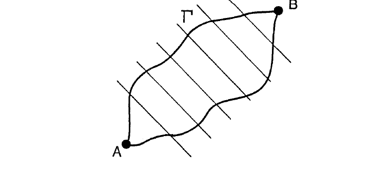
The number of wave crests we pass through is \[n=\frac{1}{2\pi}\int_A^B\vec{k}\cdot d\vec{s}.\] But since \(\oint\vec{k}\cdot d\vec{s}=\int\hat{k}\cdot\nabla\times\vec{k}\,dr=0\) (by Stokes’ theorem where \(\hat{k}\) is the unit vector normal to the surface and \(dr\) is an element of the area inside the path), then the number of wave crests inside the region is conserved. That is, the crests have no ends, so the number of crests within a wave group will be the same for all time. This need not be true for all waves, but it is true for slowly varying plane waves as defined above.
From the definition of \(\vec{k}\) and \(N\), it follows that \[\left.\frac{\partial\vec{k}}{\partial t}\right|_{\vec{x}} +\left.\nabla N\right|_t=0.\]
(1.1)
Now with the above definition of \(n\), we have \[\frac{\partial n}{\partial t} =\frac{1}{2\pi}\int_A^B\frac{\partial\vec{k}}{\partial t}\cdot d\vec{s} =-\frac{1}{2\pi}\int_A^B\nabla N\cdot d\vec{s} =\frac{1}{2\pi}(N_A-N_B).\] This says that the rate of change of the number of wave crests between \(A\) and \(B\) is equal to the rate of crest inflow at \(A\) minus the rate of crest outflow at \(B\). Thus (1.1) expresses the conservation of wave crests between \(A\) and \(B\), i.e., crests are neither created nor destroyed.
So far, we have defined the local wavenumber and frequency only as derivatives of \(\Theta\). There has been no direct statement of dynamics. We introduce dynamics by asserting that the wavenumber and frequency must be related in just the same way that they are for a plane wave! \[N=\Omega(\vec{k};\vec{x},t)\] where, if we solved for plane waves \(e^{i(\vec{k}\cdot\vec{x}-\sigma t)}\) while keeping all variable medium parameters momentarily constant, we would obtain \(\sigma=\Omega(\vec{k};\vec{x},t)\) as our dispersion relation. This turns out to be equivalent to the lowest order of a WKB calculation, despite being stated here as an arbitrary recipe.
Now this assertion and the definitions of \(\vec{k}\) and \(N\) allow us to introduce the group velocity in another way. \[\left.\frac{\partial N}{\partial t}\right|_{\vec{x}} =\left.\frac{\partial\Omega}{\partial t}\right|_{\vec{k},\vec{x}} +\left.\frac{\partial\Omega}{\partial k_i}\right|_{\vec{x},t} \left.\frac{\partial k_i}{\partial t}\right|_{\vec{x}} =\left.\frac{\partial\Omega}{\partial t}\right|_{\vec{k},\vec{x}} -c_{g_i}\left.\frac{\partial N}{\partial x_i}\right|_t\] in which the group velocity has been defined as \[c_{g_i}=\frac{\partial N}{\partial k_i}=\frac{\partial\Omega}{\partial k_i}.\]
and the repeated index implies summation. In vector form, we have \[\frac{\partial N}{\partial t}+\vec{c}_g\cdot\nabla N =\left.\frac{\partial\Omega}{\partial t}\right|_{\vec{k},\vec{x}}.\]
(1.2)
In a similar manner starting with (1.1) \[\frac{\partial k_i}{\partial t} +\frac{\partial\Omega}{\partial x_i} +\frac{\partial\Omega}{\partial k_j} \frac{\partial k_j}{\partial x_i}=0.\] Since \(\nabla\times\vec{k}=0\), then \(\partial k_j/\partial x_i=\partial k_i/\partial x_j\), so we have \[\frac{\partial k_i}{\partial t}+\vec{c}_g\cdot\nabla k_i =-\left.\frac{\partial\Omega}{\partial x_i}\right|_{\vec{k},t}.\]
(1.3)
We thus have very simple expressions, (1.2) and (1.3), for the evolution of local wavenumber \(\vec{k}\) and local frequency \(N\) as we move along a ray (i.e., we move at the local group velocity \(\vec{c}_g\)) in terms of the plane wave dispersion relation. Such variations occur when \(\Omega(\vec{k};\vec{x},t)\) has parametric \(\vec{x},t\) dependence such as if waves move in water of variable depth.
The implications of these equations deserve some discussion. Suppose first that the medium is homogeneous, i.e. \(N=\Omega(\vec{k})\ne\Omega(\vec{k};\vec{x},t)\). One possible solution is the plane wave \(\phi=ae^{i(\vec{k}\cdot\vec{x}-Nt)}\) when \(\vec{k}\) and \(N\) are constants. The initial condition is \(\phi(\vec{x},0)=ae^{i\vec{k}\cdot\vec{x}}\). Since \(\partial k_i/\partial x_j=0\) and \(\partial\Omega/\partial x_i=0\), then from (1.3), \(\partial k_i/\partial t=0\) everywhere, that is \(\vec{k}\) never changes at future times. Similarly, \(N=\Omega(\vec{k})\) gives \(N\) at \(t=0\). Since \(\partial N/\partial x_i=0\), \(\partial\Omega/\partial t=0\), then by (1.2) \(\partial N/\partial t=0\) everywhere, that is \(N\) never changes at future times. The plane wave in a homogeneous medium is thus entirely consistent with the ray theory formulation.
Suppose now that the medium remains homogeneous, but the initial conditions are more complicated. Both \(a\) and \(\vec{k}\) have slow \(\vec{x}\) dependence at \(t=0\) as illustrated below:
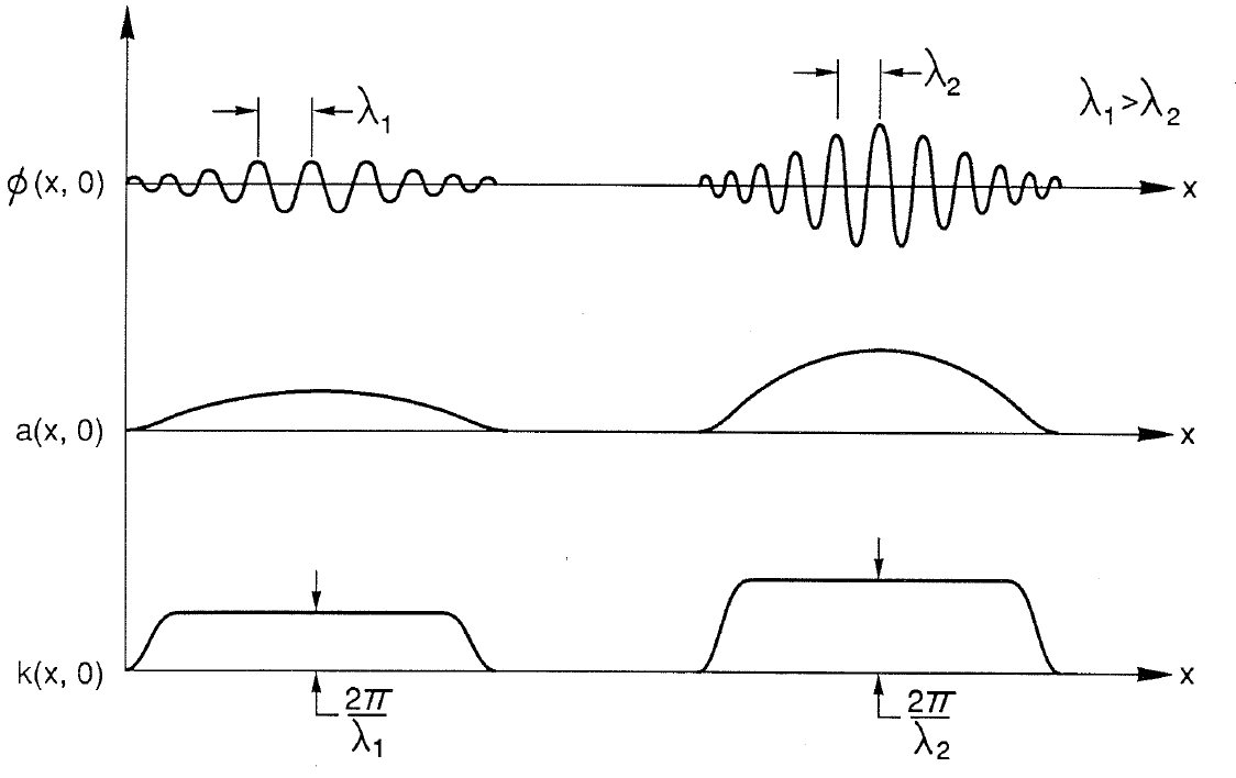
Notice that \(a\) and \(\vec{k}\) should vary slowly over \(\lambda\), even though the sketch is not very slowly varying.
The initial frequency is obtained from \(N(\vec{x},0)=\Omega[\vec{k}(\vec{x},0)]\). To find \(N(\vec{x},t)\), \(\vec{k}(\vec{x},t)\) we solve the initial value problem \[\frac{\partial k_i}{\partial t} +c_{g_j}\frac{\partial k_i}{\partial x_j}=0\] \[\frac{\partial N}{\partial t} +c_{g_j}\frac{\partial N}{\partial x_j}=0\] because the assumed homogeneity of the medium implies \(\partial\Omega/\partial t=0\) and \(\partial\Omega/\partial x_i=0\). This initial value problem may have to be solved numerically, but the equations have a simple physical interpretation. They say that, if we move at the group velocity \(\vec{c}_g=\nabla_{\vec{k}}\Omega\) appropriate to the wavenumber \(\vec{k}\) and the frequency \(N=\Omega(\vec{k})\), then we shall see no change in \(N\) and \(\vec{k}\) at future times. In other words, \(N\) and \(\vec{k}\) are constant following a group in a homogeneous medium. The situation can be sketched as follows
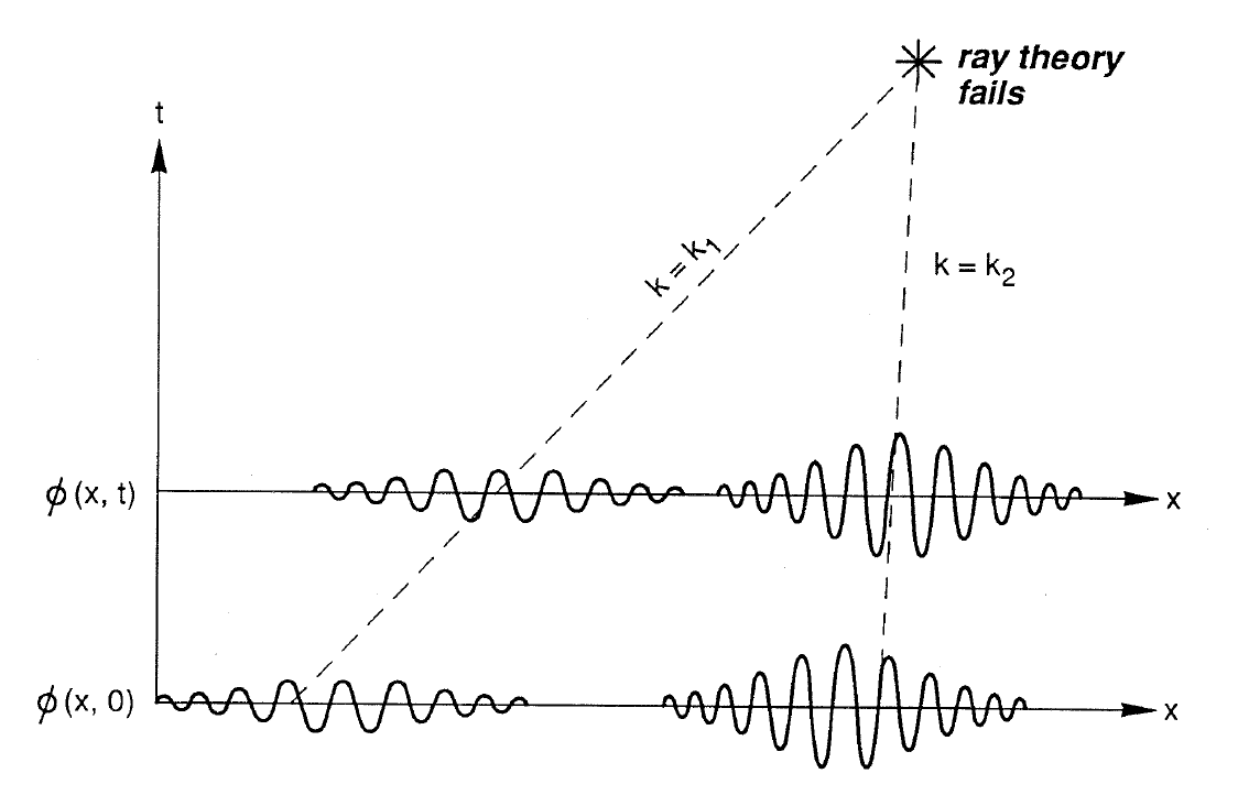
Clearly, if we sit at a fixed \(\vec{x}\), different groups pass at different times. So at fixed \(\vec{x}\), \(\partial N/\partial t\ne0\), \(\partial\vec{k}/\partial t\ne0\), in general, even though the medium is homogeneous. The whole idea fails if the rays, given by \[\vec{x}=\vec{x}_0+ \int_0^t\vec{c}_g[\vec{k}(\vec{x},t)]\,dt\] cross each other. In that case, the solution is no longer of slowly varying form.
From this point of view, the medium inhomogeneities are only technical complications. In the general inhomogeneous case, we must solve (1.2) and (1.3), so \(\vec{k}\) and \(N\) vary even though we move with a group. If we define a ‘total’ derivative as \[\frac{d}{dt}=\frac{\partial}{\partial t}+\vec{c}_g\cdot\nabla\] which is the derivative following the wave group (or wave packet), then (1.2) and (1.3) can be rewritten as \[\frac{dk_i}{dt}=-\frac{\partial\Omega}{\partial x_i}\] and \[\frac{dN}{dt}=\frac{\partial\Omega}{\partial t}.\]
while the position of the wave group is given by \[\frac{d\vec{x}}{dt}=\vec{c}_g[\vec{k}(\vec{x},t)].\] Then we have a set of three ordinary differential equations for \(\vec{x}\) (position of the wave packet), \(\vec{k}\) and \(N\). These may be integrated in time from a number of different starting positions \(\vec{x}_0\) in order to get \(\vec{k}\), \(N\) at future times, a procedure which is computationally efficient and effective. The path \(d\vec{x}/dt=\vec{c}_g\) defines the ray.
The lowest order of the corresponding WKB calculation justifies the foregoing assertions. The next order of the WKB calculation fixes the amplitude. In many cases, the more complex WKB calculation amounts to solving \[\frac{\partial\mathcal{A}}{\partial t} +\nabla\cdot(\vec{c}_g\mathcal{A})=0\] where \(\mathcal{A}=\mathcal{E}/N\) and \(\mathcal{E}\) is the wave energy. \(\mathcal{A}\) is called the action of the wave. Usually \(\mathcal{E}\propto a^2\) so this equation really describes \(a\), but a great deal of further discussion is necessary to establish its validity. Here we have simply set forward ‘recipes’ which give \(a\), \(N\), \(\vec{k}\).