Chapter 5
Shallow water dynamics
We have seen in the previous two chapters that low-frequency waves tend to have primarily horizontal motions, and their wavelengths tend to be long compared to the water depth. This allows the vertical acceleration in the vertical momentum equation to be ignored giving the hydrostatic approximation, which is equivalent to assuming that the wave frequency is much less than the buoyancy frequency, \(\sigma\ll N\). These cases may be grouped collectively under the heading of shallow water dynamics. In this chapter, we will exploit these simplifications in order to study several types of waves in detail.
Laplace’s tidal equations
Until now, we have considered the equations of motion in Cartesian coordinates only. As a preliminary step toward our study of shallow water dynamics, we consider next the effects of the earth’s curvature by examining the equations of motion in spherical coordinates.
For rotating, stratified flow on a gravitating sphere, the linearized equations of motion are \[\begin{aligned} u_t-2\Omega\sin\theta\,v+2\Omega\cos\theta\,w & =-\frac{p_\phi}{\rho_0a\cos\theta}, \\ v_t+2\Omega\sin\theta\,u & =-\frac{p_\theta}{\rho_0a}-\Omega^2a\sin\theta\cos\theta, \\ w_t-2\Omega\cos\theta\,u & =-\frac{p_z}{\rho_0}-\frac{g\rho}{\rho_0}+\Omega^2a\cos^2\theta, \\ \rho_t+w\rho_{0z} & =0, \\ u_\phi+(v\cos\theta)_\theta+a\cos\theta\,w_z & =0. \end{aligned}\] The spherical system is sketched as
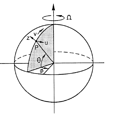
The coordinates are \[\begin{aligned} \phi & \equiv \text{longitude of the considered point }P, \\ \theta & \equiv \text{latitude}, \\ u & \equiv \text{east-west velocity}, \\ v & \equiv \text{north-south velocity}, \\ w & \equiv \text{velocity in radially upward }z\text{ direction}, \\ a & \equiv \text{earth's radius}. \end{aligned}\] These equations have already been specialized in the sense that the fluid has been assumed thin compared to the earth’s radius, i.e. \(\Delta r\ll a\), so that \(a\) could be substituted for \(r\) in all of the coefficients.
The radial and north-south momentum equations contain the centrifugal forces of the earth’s rotation as their last terms. These may be written as the gradient of a centrifugal potential, \(\nabla(\tfrac12\Omega^2\cos^2\theta\,r^2)\). This reminds us then that the solid earth and the ocean surface are not spherical surfaces, but rather equipotential surfaces of the total potential \[gr+\frac12\Omega^2\cos^2\theta\,r^2\] which is nearly spheroidal. If we worked in spheroidal coordinates, the only nonzero part of the potential gradient would be the part normal to the (equipotential) spheroidal surface. This would be a ‘gravity’ which varies by about 0.3% (\(\equiv100\times\Omega^2a/2g\)) from the poles to the equator. We shall neglect this variation of gravity with latitude and approximate the spheroidal surfaces with spherical ones. That is, we shall neglect the small centrifugal potential.
This neglect is valid on the sphere for geophysical flows rotating with the earth at speed \(\Omega\). However, in the laboratory, for rotation about the \(z\) axis, we have \[\begin{aligned} u_t-2\Omega v & =-gh_x+\frac12[\Omega^2(x^2+y^2)]_x, \\ v_t+2\Omega u & =-gh_y+\frac12[\Omega^2(x^2+y^2)]_y. \end{aligned}\] If the fluid has a free surface, then this surface will take the equilibrium shape of a paraboloid: \[h=h_0+\frac{\Omega^2}{2g}(x^2+y^2).\] If the bottom (\(z=0\)) is flat, then we must write the continuity equation as \[h_t+\nabla\cdot\left\{\vec u\left[h_0+\frac{\Omega^2}{2g}(x^2+y^2)\right]\right\}=0.\] In this case, the neglect of the centrifugal terms produces the standard shallow water equations which we have already seen. However, depending on the rotation rate and
the size of the laboratory apparatus, the centrifugal terms may not be small, so the results of the calculation may have large errors. The neglect of the centrifugal terms is really most useful for local models on the spherical earth, rather than for laboratory models.
Besides the familiar Coriolis terms, \(f=2\Omega\sin\theta\), the momentum equations contain other Coriolis terms, \(2\Omega\cos\theta\). These are due to the horizontal components of the rotation vector. They are inconvenient because they generally make the solution unseparable. If we proceed as before, assuming time dependence of \(e^{-i\sigma t}\), and combine the radial momentum equation with the density equation, we find \[(N^2-\sigma^2)w+2\Omega\cos\theta(i\sigma u)=i\sigma p_z/\rho_0\] which, when combined with the east-west (\(\phi\)) momentum equation becomes \[(N^2-\sigma^2)w+(4\Omega^2\cos^2\theta)w =i\sigma p_z/\rho_0+(4\Omega^2\sin\theta\cos\theta)v -2\Omega p_\phi/(\rho_0a).\] If \(N^2\gg4\Omega^2\), as is usually the case in the ocean, then the first term is much greater than the second term. We can then neglect the second term, which amounts to neglecting \((2\Omega\cos\theta)w\) in the east-west momentum equation. If we neglect one horizontal Coriolis term, we should neglect both because energy is conserved with both or with neither but not with just one. The neglect of the other Coriolis term in the radial momentum equation is called the traditional approximation. In some sense, we drop the \((2\Omega\cos\theta)\) because vertical buoyancy forces are much greater than vertical Coriolis forces. Again, this approximation may not be acceptable for a laboratory experiment.
Having neglected the horizontal components of rotation, \((2\Omega\cos\theta)\), we have \[u_t-2\Omega\sin\theta\,v=-\frac{p_\phi}{\rho_0a\cos\theta}\]
\[\begin{aligned} v_t+2\Omega\sin\theta\,u & =-\frac{p_\theta}{\rho_0a}, \\ w_t & =-\frac{p_z}{\rho_0}-\frac{g\rho}{\rho_0}, \\ \rho_t+w\rho_{0z} & =0, \\ u_\phi+(v\cos\theta)_\theta+a\cos\theta\,w_z & =0, \end{aligned}\] with boundary conditions \[\begin{aligned} p_t+w p_{0z}=p_t-gw\rho_0 & =0 & & \text{at }z=0, \\ w & =0 & & \text{at }z=-D. \end{aligned}\] We can separate variables as follows \[\begin{aligned} u & =e^{-i\sigma t}U(\phi,\theta)F(z), \\ v & =e^{-i\sigma t}V(\phi,\theta)F(z), \\ w & =e^{-i\sigma t}W(\phi,\theta)G(z), \\ p & =e^{-i\sigma t}P(\phi,\theta)H(z). \end{aligned}\] The equations of motion become \[\begin{aligned} (-i\sigma U-2\Omega\sin\theta\,V)F & =-\frac{P_\phi H}{\rho_0a\cos\theta}, \\ (-i\sigma V+2\Omega\sin\theta\,U)F & =-\frac{P_\theta H}{\rho_0a}, \\ (N^2-\sigma^2)WG & =\frac{i\sigma P H_z}{\rho_0}, \\ U_\phi F+(V\cos\theta)_\theta F+a\cos\theta\,WG_z & =0, \\ -i\sigma PH-g\rho_0WG & =0 & & \text{at }z=0, \\ WG & =0 & & \text{at }z=-D, \end{aligned}\] where the density equation has been combined with the radial momentum equation. The separation is completed by choosing \[W=-i\sigma P,\qquad H=g\rho_0F,\qquad G_z=F/d.\]
which results in \[\begin{aligned}-i\sigma U-2\Omega\sin\theta\,V &=-\frac{gP_\phi}{a\cos\theta},\\ -i\sigma V+2\Omega\sin\theta\,U &=-\frac{gP_\theta}{a},\\ -i\sigma P+\frac{d_n}{a\cos\theta} [U_\phi+(V\cos\theta)_\theta]&=0,\\ G_{zz}+\frac{N^2-\sigma^2}{g d_n}G&=0,\\ G_z-\frac{1}{d_n}G&=0 &&\text{at }z=0,\\ G&=0 &&\text{at }z=-D.\end{aligned}\]
(5.1)
The first three equations contain variables which depend on \(\phi\) and \(\theta\) only. That is, they contain all of the horizontal dependence of \(u,v,w\) and \(p\). The vertical dependence is entirely contained in the fourth equation which, along with the boundary conditions, is an eigenvalue problem in which \(d_n^{-1}\) is the eigenvalue. The eigenfunction determines the vertical variation of \(w\) and, indirectly, of \(u,v\) and \(p\).
There is an infinite number of sets of horizontal structure equations, each set being identical except that instead of the total water depth \(D\), each system now has an equivalent depth \(d_n\). The lowest equivalent depth \(d_0\) is effectively the actual (constant) depth. The higher equivalent depths go like \(1/n^2\) and correspond to the \(n\)th mode vertical variations of \(w\). The equations for \(U,V\) and \(P\) are called Laplace’s Tidal Equations or LTE.
Notice that the separation of variables fails if the bottom is not flat because we no longer get an eigenvalue problem in \(z\). But if the bottom is flat to a good approximation, then LTE give the horizontal variation of both surface and internal modes providing we interpret \(d_n\) properly. That is, \(d_0\) gives the surface gravity mode while \(d_n\) give the internal gravity modes.
For free oscillations, only those \(d_n>0\) have physical significance. But the eigenvalue problem for \(G\) may also have negative \(d_n\). These correspond to modes which are evanescent in the horizontal. They may be excited in forced solutions of LTE.
Shallow water equations with rotation
If we neglect the centrifugal acceleration terms, make the traditional approximation and consider motions with horizontal and vertical scales which are small compared to the earth’s radius, then the equations of motion may be written in Cartesian coordinates as \[\begin{aligned} u_t-fv & =-\frac{1}{\rho_0}p_x, \\ v_t+fu & =-\frac{1}{\rho_0}p_y, \\ 0 & =-\frac{1}{\rho_0}p_z-\frac{g\rho}{\rho_0}, \\ \rho_t+w\rho_{0z} & =0, \\ u_x+v_y+w_z & =0, \end{aligned}\] where the flow has been assumed hydrostatic, i.e. \(w_t\) has been neglected, and \(f=2\Omega\sin\theta\). Remember also that the density has been separated into a background part which varies in \(z\) only and a perturbation, \(\rho^*=\rho_0(z)+\rho(x,y,z,t)\) where \(\rho\ll\rho_0\). Then the hydrostatic part has been subtracted and the Boussinesq approximation has been made allowing the function \(\rho_0(z)\) to be considered constant everywhere except in the density equation. The vertical momentum equation and the density equation can be combined to yield \[N^2w=-\frac{1}{\rho_0}p_{zt}.\]
Consider first the case of a homogeneous fluid in which \(\rho=0\). The vertical momentum equation is the hydrostatic relation \(p_z=-g\rho_0\) (\(p\) is now total pressure), which when integrated yields \[p|_\eta-p(z)=-g\rho_0(\eta-z)\] from which \[p(z)=p_{atm}+g\rho_0(\eta-z).\] We shall assume that the atmospheric pressure is zero, so \[p(z)=g\rho_0(\eta-z).\] We see that the horizontal pressure gradient is independent of \(z\), so the equations of motion can be written \[\begin{aligned} u_t-fv & =-g\eta_x, \\ v_t+fu & =-g\eta_y, \\ u_x+v_y+w_z & =0. \end{aligned}\] Integrating continuity from \(z=-D\) to \(z=\eta\) yields \[\int_{-D}^{\eta}(u_x+v_y)\,dz+w|_{z=\eta}-w|_{z=-D}=0.\] Since \(u\) and \(v\) are not functions of \(z\), then this becomes \[(u_x+v_y)(\eta+D)+w|_{z=\eta}-w|_{z=-D}=0.\] The top and bottom boundary conditions are \[w=\frac{D\eta}{Dt}\quad\text{at }z=\eta \ ;\qquad w=-uD_x-vD_y\quad\text{at }z=-D.\] Combining these with continuity yields \[\eta_t+[u(\eta+D)]_x+[v(\eta+D)]_y=0.\]
If we assume that the surface deviations are much smaller than the water depth, i.e. \(\eta\ll D\), then the final linearized set of equations is \[\begin{aligned}u_t-fv&=-g\eta_x,\\ v_t+fu&=-g\eta_y,\\ \eta_t+[uD]_x+[vD]_y&=0.\end{aligned}\]
(5.2)
These are the linear shallow water equations with rotation. We derived the nonrotating version with constant depth in the chapter on surface gravity waves. Notice that, for constant depth \(D\), they have the same form as LTE but written in Cartesian coordinates.
Now return to the equations with stratification included. As we did in the previous section, if the depth is constant, we may separate variables as \[\begin{aligned} u & =U(x,y,t)F(z), \\ v & =V(x,y,t)F(z), \\ w & =W(x,y,t)G(z), \\ p & =P(x,y,t)H(z). \end{aligned}\] The equations become \[\begin{aligned} (U_t-fV)F & =-\frac{1}{\rho_0}P_xH, \\ (V_t+fU)F & =-\frac{1}{\rho_0}P_yH, \\ N^2WG & =-\frac{1}{\rho_0}P_tH_z, \\ (U_x+V_y)F+WG_z & =0. \end{aligned}\] If we choose \[H=g\rho_0F\ ;\qquad G_z=F/d\ ;\qquad W=P_t\]
then the equations reduce to \[\begin{aligned} U_t-fV & =-gP_x, \\ V_t+fU & =-gP_y, \\ P_t+d_n(U_x+V_y) & =0, \\ G_{zz}+\frac{N^2(z)}{g d_n}G & =0, \\ G_z-\frac{1}{d_n}G & =0 & & \text{at }z=0, \\ G & =0 & & \text{at }z=-D. \end{aligned}\] The boundary condition at \(z=0\) comes from \(p=g\rho_0\eta\) at \(z=0\). Differentiating with respect to time yields \(\partial p/\partial t=g\rho_0\partial\eta/\partial t=g\rho_0w\) or \(H\partial P/\partial t=g\rho_0WG\) from which the boundary condition follows.
As in the previous section on LTE, we have separated the horizontal dependence into a set of three equations which are identical to the linear shallow water equations for a flat-bottom ocean. As before, the pressure plays the part of the sea-surface displacement. The vertical structure is entirely contained in an eigenvalue problem in which \(d_n^{-1}\) are the eigenvalues. These are again the equivalent depths to be used in the horizontal structure equations. Note that we have not had to assume a periodic time dependence here because the hydrostatic approximation has eliminated the vertical acceleration which previously showed up in the equation for \(G\) as the \(\sigma^2\) in the coefficient. That is, the hydrostatic approximation, in this case, is the same as assuming \(\sigma^2\ll N^2\).
The real point here is that, in a flat-bottom ocean, stratification makes possible an infinite sequence of internal replicas of the barotropic, long, shallow water gravity waves. The horizontal variations of these internal modes are described by the same equations that describe the barotropic mode, except that the equivalent depth \(d_n\)
replaces the total depth \(D\). These modes are uncoupled, so we can solve each set of equations separately and add them to find a more general solution. Without rotation, the speed of long barotropic waves is \((gd_0)^{1/2}\simeq200\ \mathrm{m\,s^{-1}}\) in the deep sea. Long internal gravity waves move at the much slower speed of \((gd_n)^{1/2}\simeq1/n\ \mathrm{m\,s^{-1}}\). Thus for comparable frequencies, the internal waves have much shorter wavelengths than the surface barotropic mode.
It is appropriate at this point to ask “What exactly does \(d_n\) represent?” After all, each \(d_n\) is much smaller than the vertical scale associated with the vertical mode \(n\). One way to understand the \(d_n\) is first to write the buoyancy frequency as \[N=(g/h)^{1/2} \qquad\text{where}\qquad h=-(\rho_{0z}/\rho_0)^{-1}=g/N^2\] which is the density scale height, i.e. the vertical scale over which the background density varies. This scale height is typically much greater than the ocean depth. For constant \(N\), the equation for \(d_n\) can now be written as \[\tan\left(\frac{D}{(hd_n)^{1/2}}\right) =\left(\frac{d_n}{h}\right)^{1/2}\] from which it is clear that the rigid lid approximation applies when \(d_n/h\ll1\). In this case, the vertical wavenumber for mode \(n\) is given by \(n\pi/D=(hd_n)^{-1/2}\) which leads to a vertical scale of \(\lambda_v=2\pi(hd_n)^{1/2}\). Rewritten, this becomes \[d_n=\frac{\lambda_v^2}{4\pi^2h}\] which says that \(d_n\) is proportional to the square of the vertical scale of mode \(n\) divided by the density scale height. For \(n>1\), this quantity is typically small, so \(d_n\) is small as well. Another way to view this is that the vertical scale of the mode is proportional to the geometric mean of the density scale height and the equivalent depth, i.e. \(\lambda_v\propto(hd_n)^{1/2}\).
The simplicity of these flat-bottom results is not extendable to the case of variable bottom topography. However, we should keep in mind that, when considering the flat-bottom ocean, all of the long shallow water barotropic waves which we are about to study on the \(f\)-plane have an infinite number of internal replicas allowed by stratification.
Reflection at a solid wall
We consider first several types of waves which can exist in the absence of rotation. Therefore, we take \(f=0\) and the equations are \[\begin{aligned} u_t & =-g\eta_x, \\ v_t & =-g\eta_y, \\ \eta_t+D(u_x+v_y) & =0. \end{aligned}\] Free wave solutions have the form \(\eta=e^{-i\sigma t+ikx+i\ell y}\) which leads to \[u=\frac{gk}{\sigma}\eta \ ;\qquad v=\frac{g\ell}{\sigma}\eta.\] Substitution into continuity gives the dispersion relation \[\sigma^2=gD(k^2+\ell^2)=gDK^2.\]
(5.3)
These are nothing more than surface gravity waves in shallow water which are nondispersive with \[c=\sigma/K=(gD)^{1/2} \ ;\qquad |\vec c_g|=d\sigma/d|\vec k|=(gD)^{1/2}.\]
Suppose the wave is incident upon a solid wall at \(x=0\).
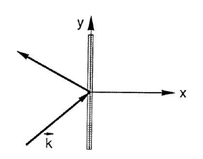
The velocity normal to the wall must vanish, i.e. \(u=0\) at \(x=0\). The total solution may be constructed by adding a reflected wave with the same amplitude and no phase shift \[\eta =a e^{-i\sigma t+ikx+i\ell y} +a e^{-i\sigma t-ikx+i\ell y}.\] The angle of reflection, \(\alpha=\tan^{-1}(\ell/k)\), is equal to the angle of incidence, i.e. the reflection is specular.
Seiches in a box
Now consider a domain bounded by four solid walls.
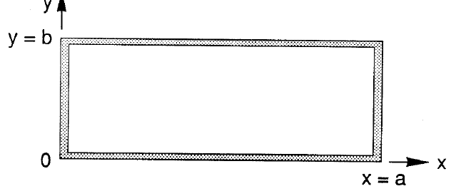
We assume a periodic time dependence of \(e^{-i\sigma t}\) so that the equations become \[\begin{aligned} -i\sigma u & =-g\eta_x, & -i\sigma v & =-g\eta_y, \\ -i\sigma\eta+D(u_x+v_y) & =0. \end{aligned}\] (Note that \(\eta\) is now different from the full \(\eta\) because of the removal of the time dependence. We should write the new variables with a hat or something, like \(\hat{\eta}\), but
this gets cumbersome. So, we rely on our memory to reconstruct the full variables— not a good practice for any formal problem solving.) We can eliminate \(u\) and \(v\) to find an equation for the surface elevation \[\nabla^2\eta+\frac{\sigma^2}{gD}\eta=0.\] If \(\eta=e^{ikx+i\ell y}\), then we recover the previous solutions. However, in the box domain, the velocity normal to each boundary must vanish. From the momentum equations, this requires \[\begin{aligned} \eta_x & =0 & & \text{at }x=0,a, \\ \eta_y & =0 & & \text{at }y=0,b. \end{aligned}\] The solution is then \[\eta =\cos\left(\frac{n\pi x}{a}\right) \cos\left(\frac{m\pi y}{b}\right), \qquad n,m=0,1,\ldots\] When substituted into the equation for \(\eta\), we get \[\sigma^2 =gD\left(\frac{n^2}{a^2}+\frac{m^2}{b^2}\right)\pi^2.\]
(5.4)
These are the normal, or free modes, of the nonrotating basin. They are standing waves with \(n,m\) zero crossings in \(\eta\) across the basin. Suppose the basin is forced by an external force, say the wind, and then the wind suddenly stops. During the time the wind is blowing, water is piled up at one extremity of the basin, thus creating a pressure gradient. When the wind stops, there is nothing to balance the pressure gradient, so the water begins to flow down it. There is no friction, so the water overshoots its equilibrium position of a flat surface, and begins to pile up on the other side of the basin. This process continues indefinitely (or until friction damps out the motions in a real fluid). These oscillations are called seiches (pronounced “say shez”).
The gravest mode \(m=0\), \(n=1\); \(\eta=\cos(\pi x/a)\) has the lowest frequency \(\sigma^2=gD\pi^2/a^2\) and has a period of \(T=2\pi/\sigma=2a/(gD)^{1/2}\), i.e. the period is the time required for a wave to cross the basin (0 to \(a\)) and go back again. It has one nodal line at \(x=a/2\). All other modes have one or more nodal lines and their frequencies are greater than that of the gravest mode.
Quite generally, for a basin of arbitrary shape, the Neumann problem for the Helmholtz equation \[\nabla^2\eta+(\sigma^2/gD)\eta=0 \ ;\qquad \partial\eta/\partial n=0 \quad\text{at boundaries}\] results in a sequence of free periods \(\sigma_1^2,\sigma_2^2,\sigma_3^2,\ldots\) having a positive lowest member and no upper limit.
Propagation over a step
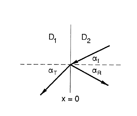
Consider a free wave encountering a step change in depth.
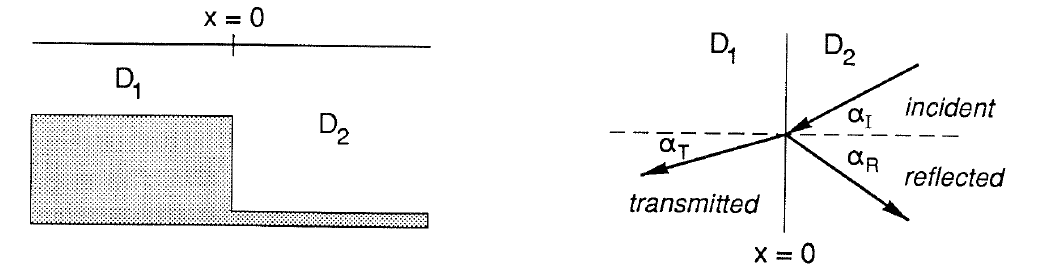
This can be thought of as a shelf of infinite width. At the step, there are two new waves which can be generated. One is a reflected wave and one is a transmitted wave. In a sense, the step acts as a permeable or leaky wall rather than a solid wall. There are no variations along the step in the \(y\) direction, so we may assume that all three waves have the same alongstep wavenumber, as well as the same frequency. Thus, \(\eta\)
must go like \(e^{-i\sigma t-i\ell y}\), so the solutions on each side of the step are \[\begin{aligned} x<0\qquad \eta & =e^{-i\sigma t-i\ell y}\left(A_Te^{-ik_1x}\right), \\ x>0\qquad \eta & =e^{-i\sigma t-i\ell y} \left(A_Ie^{-ik_2x}+A_Re^{ik_2x}\right), \end{aligned}\] where the amplitudes \(A_{I,R,T}\) are unknown. To find the unknown amplitudes, we must require that the solution is consistent across the step. Without proof, this can be accomplished by matching the sea-surface displacement (\(\eta\)) and the across-step transport (\(uD\)) on each side of the step. Thus, at \(x=0\), we require \[\begin{aligned} A_I+A_R & =A_T, \\ D_2k_2(-A_I+A_R) & =D_1k_1(-A_T). \end{aligned}\]
Before proceeding, we should note that this matching of transport completely ignores the fact that flow should not occur through the vertical section of the step. In fact, the present solution necessarily imposes a flow through the vertical part unless the horizontal velocity goes to zero at \(x=0\) (because there is no vertical variation, so if the velocity is nonzero at the surface, then it is nonzero at depth). This apparent inconsistency can be resolved by considering the full equations without the shallow water approximation. The complete solution is quite complicated near the step, but the shallow water solution is recovered far away from the step (Bartholomeusz, 1958). The present solution also conserves energy, which was enough to convince Lamb (1832) that the results were correct. There are problems, however, in which the simple matching of pressure and transport leads to erroneous results.
To continue, the matching allows the reflected and transmitted amplitudes to be written in terms of the incident amplitude \[A_T=2A_I/(1+D_1k_1/D_2k_2).\]
(5.5)
\[A_R=A_I(1-D_1k_1/D_2k_2)/(1+D_1k_1/D_2k_2).\]
(5.6)
Notice that, if \(D_1\to0\), then \(A_R=A_I\) which is reasonable. But \(A_T=2A_I\) which appears incorrect. This occurs because the shallow side of the step does not vanish unless the depth is identically zero. Otherwise, the transmitted amplitude simply gets larger. If \(D_1=D_2\), then \(A_T=A_I\) and \(A_R=0\), both of which are sensible. If we define the total wavenumbers as \[\begin{aligned} K_I=K_R & =(k_2^2+\ell^2)^{1/2}=\sigma/(gD_2)^{1/2}, \\ K_T & =(k_1^2+\ell^2)^{1/2}=\sigma/(gD_1)^{1/2}, \end{aligned}\] then, \[\ell=K_I\sin\alpha_I=K_R\sin\alpha_R,\] \[\alpha_I=\alpha_R,\] so the reflection is specular. Since \[\ell=K_I\sin\alpha_I=K_T\sin\alpha_T,\] \[\frac{\sin\alpha_I}{(gD_2)^{1/2}} =\frac{\sin\alpha_T}{(gD_1)^{1/2}},\] \[\frac{\sin\alpha_I}{c_I}=\frac{\sin\alpha_T}{c_T},\]
(5.7)
which is Snell’s law. Because \(D_1<D_2\), then \(\sin\alpha_T<\sin\alpha_I\) so waves are refracted towards normal incidence (\(\alpha_T=0\)).
Now suppose that the incident wave arrives from the shallow side of the step.
In this case, the reflected and transmitted amplitudes are still given by the above formulas and Snell’s law still holds. As \(\alpha_I\) increases, \(\alpha_T\) increases even faster since \(\alpha_T>\alpha_I\). Eventually, a critical angle of incidence, \(\alpha_I'\), is reached where \(\alpha_T=90^\circ\).
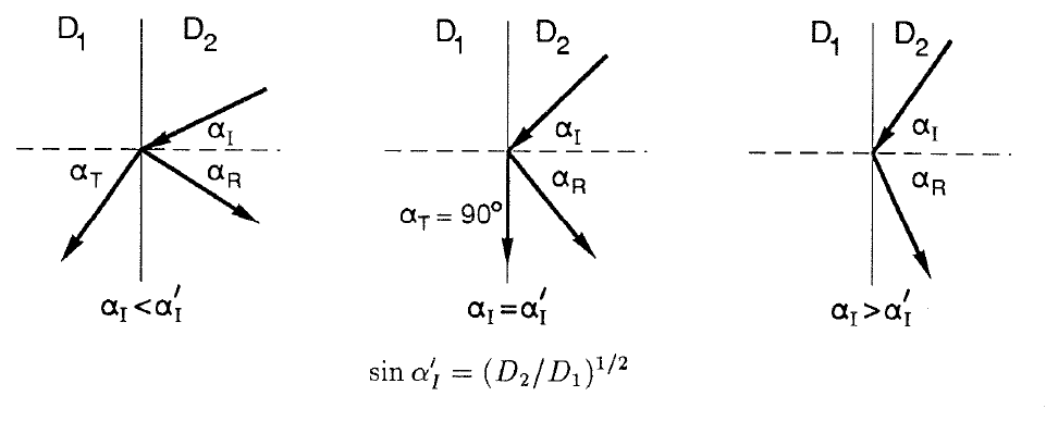
\[\sin\alpha_I'=\left(\frac{D_2}{D_1}\right)^{1/2}.\]
(5.8)
For \(\alpha_I=\alpha_I'\), \[\ell=K_I\sin\alpha_I =\frac{\sigma}{(gD_2)^{1/2}} \frac{D_2^{1/2}}{D_1^{1/2}} =\frac{\sigma}{(gD_1)^{1/2}} =K_T,\] so \(k_1=0\). For \(\alpha_I>\alpha_I'\), \[\ell>K_T=(k_1^2+\ell^2)^{1/2},\] so \(k_1^2<0\), i.e. the transmitted wave decays exponentially away from the step. There is total internal reflection.
Edge waves and coastal seiches
We can use these ideas to examine waves which might occur along a continental shelf. We idealize the shallow shelf as a flat-bottom region of width \(L\). The continental slope is reduced to a step change in depth dropping down to a flat-bottom deep ocean. This is the classic step shelf.
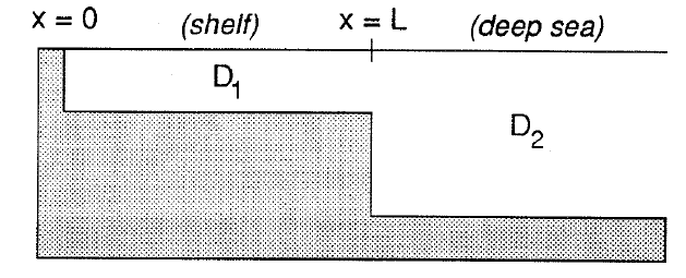
We anticipate from the foregoing that two kinds of solutions exist. They are (A) waves trapped on the shelf by critical internal reflection at the shelf edge, and (B) waves arriving from the deep sea, traversing the shelf, being reflected at the coast and finally returning to the deep sea. Ray paths for the two cases are
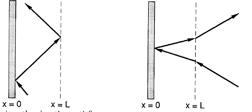
In each region, the elevation satisfies \[\nabla^2\eta+(\sigma^2/gD)\eta=0.\] We will analyze the two cases separately.
Case A: Here we write \[\begin{aligned} \eta & =A\cos k_1x & & 0<x<L, \\ \eta & =Be^{-k_2(x-L)} & & x>L, \end{aligned}\] which satisfies \(u=0\) at \(x=0\) and assumes internal reflection at the shelf edge. The cross-shelf structure looks like
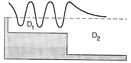
Thus, we must have \[k_1^2=\sigma^2/gD_1-\ell^2 \ ;\qquad k_2^2=\ell^2-\sigma^2/gD_2.\] Notice that both \(k_1\) and \(k_2\) are real provided \[\sigma^2/gD_1>\ell^2>\sigma^2/gD_2,\] i.e. provided \(D_1<D_2\).
Matching \(\eta\) and \(uD\) (really \(D\eta_x\)) at \(x=L\) yields \[\begin{aligned} A\cos k_1L & =B, \\ -D_1k_1A\sin k_1L & =-D_2k_2B, \end{aligned}\] from which \[\tan k_1L=k_2D_2/k_1D_1,\]
(5.9)
which, along with the definitions of \(k_1\) and \(k_2\), is effectively a relation between \(\sigma\) and \(\ell\), i.e. a dispersion relation.
The details of solving for the free waves gets a bit obscure and is usually done numerically with a root solving procedure. The solutions consist of an infinite set of wave modes which can occur between the lines \(\sigma=(gD_2)^{1/2}\ell\) and \(\sigma=(gD_1)^{1/2}\ell\).
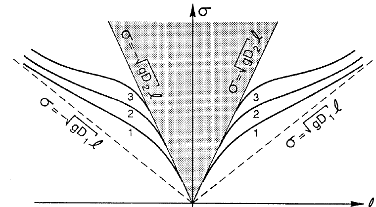
Each mode has its own ‘dispersion relation’. For large \(\ell\), \(k_1\simeq(n\pi+\pi/2)/L\), i.e. the elevation profile looks like that sketched above with \(n\) zero crossings on the shelf followed by exponential decay into the deep sea. These modes are entirely analogous to waveguide modes. The shelf break acts as a wall in some sense. If we fix the frequency, then only a finite number of propagating modes (i.e. propagating in the \(y\) direction) exist. These refractively trapped modes are called edge waves.
Case B: Here we write \[\begin{aligned} \eta & =A\cos k_1x & & 0<x<L, \\ \eta & =Be^{ik_2(x-L)}+Ce^{-ik_2(x-L)}, \end{aligned}\] which satisfies \(u=0\) at \(x=0\) and allows for incident (\(C\)) and reflected (\(B\)) deep ocean waves. The cross-shelf structure looks like
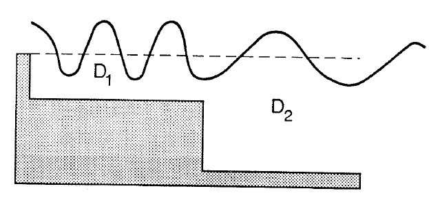
Now we must have \[k_1^2=\sigma^2/gD_1-\ell^2 \ ;\qquad k_2^2=\sigma^2/gD_2-\ell^2\] and \(\ell^2<\sigma^2/gD_2\). Matching \(\eta\) and \(uD\) at \(x=L\) yields \[\begin{aligned} A\cos k_1L & =B+C, \\ -D_1k_1A\sin k_1L & =iD_2k_2(B-C), \end{aligned}\] from which, after eliminating \(B\), \[A=C\frac{i\,2D_2k_2} {iD_2k_2\cos k_1L-D_1k_1\sin k_1L}.\]
Once again obtaining solutions is a bit obscure. Notice that the wave amplitudes do not drop out as they did for the edge waves. This is because the present solution relies on an incident wave which essentially forces the response over the shelf. There is no restriction on \(\sigma,\ell\) except that \(\ell^2<\sigma^2/gD_2\). Thus, an entire continuum of solutions exists as indicated in the above dispersion diagram.
We can get a sense of the effect of the shelf by considering the case of \(\ell=0\). Then \(D_1k_1=\sigma(D_1/g)^{1/2}\) and \(D_2k_2=\sigma(D_2/g)^{1/2}\). The magnitude of \(A/C\) becomes \[\left|\frac{A}{C}\right| =\frac{2(D_2/g)^{1/2}} {\left[(D_2/g)\cos^2k_1L+(D_1/g)\sin^2k_1L\right]^{1/2}}.\] The extrema occur where \(\partial|A/C|/\partial\sigma=0\) which happens when either \(\cos k_1L=0\) or \(\sin k_1L=0\). But, since \(D_2>D_1\), the maximum occurs when \(\cos k_1L=0\) or \[\sigma=\frac{(gD_1)^{1/2}}{L}(n\pi+\pi/2).\]
(5.10)
These are the so-called quarter-wave resonances or, in the present context, coastal seiches. They are like box seiches in that they are standing waves in the cross-shelf direction, but they have a node in elevation at the shelf break.
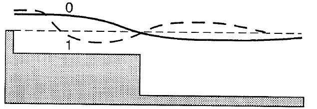
If they were forced by a wind stress, however, they would damp out rather quickly because of the loss of energy to the deep ocean. They are, therefore, sometimes called leaky edge waves.
Sverdrup and Poincaré waves
We now return to the equations of motion with rotation. We assume that the rotation rate is constant, i.e. an \(f\)-plane. Taking the time dependence again to be \(e^{-i\sigma t}\), we find \[\begin{aligned} u & =\frac{g}{\sigma^2-f^2}(f\eta_y-i\sigma\eta_x), \\ v & =-\frac{g}{\sigma^2-f^2}(f\eta_x+i\sigma\eta_y), \\ \nabla^2\eta+\frac{\sigma^2-f^2}{gD}\eta & =0, \end{aligned}\] which is analogous to the previous equations for the non-rotating case.
In the infinite domain, a plane wave has the form \(\eta=e^{ikx+i\ell y}\) which gives the dispersion relation \[\sigma^2=gD(k^2+\ell^2)+f^2.\]
(5.11)
These are long gravity waves modified by rotation, and are sometimes called Sverdrup waves. If we orient the axes so that the \(x\) direction is along the total wavenumber, then
\(\ell=0\) and \(k=|\vec{k}|\). This leads to \[u=\frac{g\eta}{\sigma^2-f^2}(\sigma k) \ ;\qquad v=\frac{g\eta}{\sigma^2-f^2}(-ifk)\] from which we see that \(u/v=i\sigma/f\). The particle motions are no longer along the wavenumber vector, but are ellipses rotating in the clockwise direction in the northern hemisphere. The ratio of major to minor axes is \(\sigma/f\).
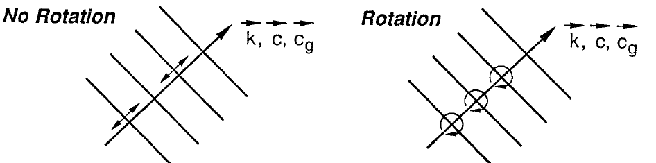
Rotation makes the waves dispersive with \[c_{gx}=\frac{gD}{\sigma}k \ ;\qquad c_{gy}=\frac{gD}{\sigma}\ell.\] The group velocity is again parallel to the wavenumber vector.
These plane waves propagate in the unbounded fluid only when \(\sigma>f\), that is \(f\) is the lowest frequency possible for them to exist. The group velocity rises from zero at \(\sigma=f\) towards an upper limit given by the non-rotating, shallow water dispersion relation. If \(\sigma\ll f\), then we can neglect \(\sigma\) with respect to \(f\). The time variation is so small that the system is quasi-steady. If \(\partial/\partial t\sim0\), then the equations of motion become \[-fv=-g\eta_x \ ;\qquad fu=-g\eta_y\] which represents steady, geostrophic motion. If \(\sigma=f\), then from \(\sigma^2-f^2=0\) it follows that \(k=0\) and \(\ell=0\), so we have \[u_t-fv=0 \ ;\qquad v_t+fu=0.\]
which has solutions \[u=\cos(\sigma t)=\cos(ft) \ ;\qquad v=\sin(\sigma t)=\sin(ft).\] These are inertial oscillations which are perfect circles always remaining in the same place.
Consider now the reflection of a Sverdrup wave from a solid wall. As in the non-rotating case, we require that the velocity normal to the wall vanish. For a wall at \(x=0\), then \(u=0\) there. This leads to \[-i\sigma\eta_x+f\eta_y=0 \qquad\text{at }x=0.\] The solution is found by adding an incident and a reflected wave, although now they may have different amplitudes. We write \[\eta=a_i e^{ikx+i\ell y}+a_r e^{-ikx+i\ell y}\] which satisfies the boundary condition provided that \[-i\sigma(ika_i-ika_r)+f(i\ell a_i+i\ell a_r)=0\] from which \[\frac{a_r}{a_i}=\frac{\sigma k-i f\ell}{\sigma k+i f\ell}.\]
(5.12)
If \(f=0\), then \(a_r=a_i\), the reflected wave has equal amplitude to that of the incident wave and there is no phase shift. With rotation, the angle of incidence \(\tan^{-1}(\ell/k)\) still equals the angle of reflection, but the reflected amplitude differs from the incident amplitude by a multiplicative constant with unit magnitude. This means that there is a phase shift upon reflection. So the waves are standing in the direction normal to the wall, reflected with a phase shift, and they are travelling along the wall. They constitute a continuum in the sense that they may occur at any frequency and wavenumber combination as long as \(\sigma>f\), i.e. the single boundary does not discretize them into modes. These waves are often called Poincaré waves.
Kelvin waves
A solid wall makes possible a rather special wave which is trapped at the wall and can propagate with \(\sigma>f\) or \(\sigma<f\). This is called a Kelvin wave and is basically a gravity wave modified by rotation. It has the peculiar property that the velocity normal to the wall is identically zero everywhere, not just at the wall. Let’s consider the wall at \(x=0\) as before. The Kelvin wave has \(u\equiv0\) which reduces the equations of motion to \[\begin{aligned} -fv & =-g\eta_x, & v_t & =-g\eta_y, \\ \eta_t+Dv_y & =0. \end{aligned}\] The velocity along the wall, \(v\), is in geostrophic balance while the \(y\) momentum equation gives the acceleration along the wall. Physically, this means that the pressure gradient along the wall created by the sea-level fluctuation produces an acceleration along the wall, but the pressure gradient normal to the wall adjusts itself at every instant so as to be in geostrophic balance with the velocity along the wall.
Assuming the standard time dependence of \(e^{-i\sigma t}\), the Kelvin wave moves along the coast satisfying \[\eta_{yy}+\frac{\sigma^2}{gD}\eta=0.\] Choosing \[\eta=a(x)e^{i\ell y}\] where \(a(x)\) is still of unknown form, the dispersion relation is \[\sigma^2=gD\ell^2\]
(5.13)
which is identical to the gravity wave dispersion relation in the absence of rotation! The function \(a(x)\) is found by combining the two momentum equations to find \[-i\sigma\eta_x+f\eta_y=0.\]
Notice that this is identical to the statement that \(u=0\) which we previously satisfied at the wall, but is now satisfied everywhere. From this we obtain an expression for \(a(x)\), namely \[a(x)=a_0e^{f\ell x/\sigma}.\] The full solution is \[\eta=a_0e^{-i\sigma t+i\ell y}e^{f\ell x/\sigma} =a_0e^{-i\sigma t\pm i\sigma y/(gD)^{1/2}\pm f x/(gD)^{1/2}}.\] If the wave is on the \(x>0\) side of the boundary, then we must require that the solution remain finite as \(x\to\infty\). This means that \(\lim_{x\to\infty}\eta\to0\) which means that \(\ell<0\). That is, the wave must travel in the \(-y\) direction in this case. If the wave were on the \(x<0\) side of the wall, then we would require that \(\ell>0\) so the wave would travel in the \(+x\) direction. Thus, the wave always travels with the wall on its right in the northern hemisphere (\(f>0\); everything is reversed if \(f<0\)). The wave amplitude decreases exponentially moving away from the wall, so the wave is trapped along the wall by rotation. A faithful drawing of a Kelvin wave may be found in Gill (1982, p.380).
Waveguide modes
Consider an infinitely long channel in the \(x\) direction with sides at \(y=0\), \(y=a\).
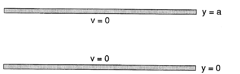
We seek to determine the kinds of waves which may propagate subject to \(v=0\) at \(y=0,a\). We must solve \[\nabla^2\eta+\frac{\sigma^2-f^2}{gD}\eta=0\] \[i\sigma\eta_y+f\eta_x=0 \qquad\text{at }y=0,a.\] Look for solutions of the form \[\eta=e^{ikx}\left( \cos\frac{m\pi y}{a}+\alpha_m\sin\frac{m\pi y}{a} \right).\] This satisfies the field equation if \[k^2=\frac{\sigma^2-f^2}{gD}-\left(\frac{m\pi}{a}\right)^2.\]
(5.14)
The boundary conditions are \[\begin{gathered} i\sigma\frac{m\pi}{a} \left(-\sin\frac{m\pi y}{a}+\alpha_m\cos\frac{m\pi y}{a}\right)\\ +ifk\left(\cos\frac{m\pi y}{a}+\alpha_m\sin\frac{m\pi y}{a}\right)=0 \qquad\text{at }y=0,a \end{gathered}\] from which \[\alpha_m=-\frac{fka}{\sigma m\pi}, \qquad m=1,2,\ldots\] There is no \(m=0\) mode because it does not satisfy the boundary condition at \(y=a\).
Notice that as \(m\) increases, \(k\) decreases and finally becomes imaginary. Only for \[m=1,2,\ldots< \left(\frac{(\sigma^2-f^2)a^2}{gD\pi^2}\right)^{1/2}\]
may these waves propagate along the channel and then only if \(\sigma^2>f^2\). They propagate in either direction. If \(\sigma^2<f^2\) or \(m>m_{max}\), then these waves decay exponentially along the channel. They are then meaningless in the infinite channel case but may represent realistic motion if the channel is walled off at some point. These are Poincaré channel modes.
Regular Kelvin waves are also possible. As earlier, we may have \[\eta=e^{-i\sigma t+i\sigma x/(gD)^{1/2}-fy/(gD)^{1/2}}\] that is, a Kelvin wave moving east along \(y=0\). We may now also have \[\eta=e^{-i\sigma t-i\sigma x/(gD)^{1/2}+f(y-a)/(gD)^{1/2}}\] that is, a Kelvin wave moving west along \(y=a\). If only one wave is excited, then the surface elevation looks like a regular gravity wave progressing up or down the channel except that the crest-trough amplitude decays to the left of the direction of propagation. Because of the non-trigonometric cross-channel variations, the superposition of two Kelvin waves travelling in opposite directions does not lead to a standing wave, but rather to motion in which the wave crests appear to rotate about amphidromic points where the rise and fall vanishes.
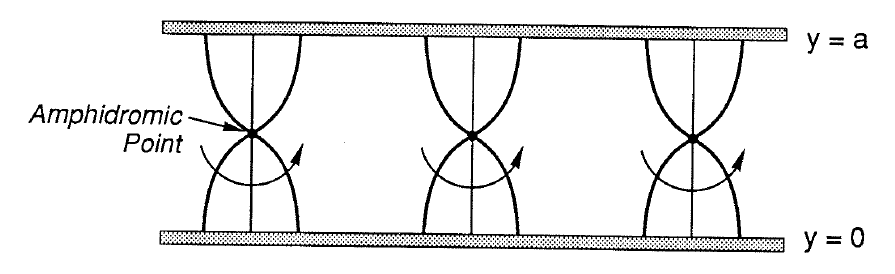
These points are separated by \(\pi/k=\pi(gD)^{1/2}/\sigma\); the crests rotate once about each amphidrome in a period \(2\pi/\sigma\).
Kelvin wave reflection
The case of a channel closed at one end is interesting, for we see how Kelvin waves are reflected.
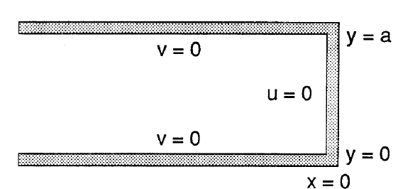
The idea is to have an incident plus an outgoing Kelvin wave. Nowhere is \(u=0\) for such a combination although \(v=0\) everywhere. We now include an infinite series of Poincaré waves, for which \(v=0\) at \(y=0,a\) and choose them so that their \(u\) at \(x=0\) just cancels that of the Kelvin waves. Without doing the analysis, we may see one result. All Poincaré waves are needed to make \(u=0\) at \(x=0\). Now if \(\sigma^2<f^2\), then all Poincaré waves decay exponentially as \(x\to-\infty\) so that, far from \(x=0\), the solution is only the incident Kelvin wave going east along \(y=0\) plus the reflected Kelvin wave going west along \(y=a\). But if \(\sigma^2>f^2\) sufficiently so that \[m_{max}=\left(\frac{(\sigma^2-f^2)a^2}{gD\pi^2}\right)^{1/2}>1\] then one or more Poincaré waves vary trigonometrically with \(x\) and the reflected wave is not a simple Kelvin wave. Clearly if \(\sigma^2>f^2\) at all, then if the channel is sufficiently wide, this will be the case. In other words, perfect reflection of a Kelvin wave occurs if \[\frac{\sigma^2-f^2}{gD}<\frac{\pi^2}{a^2}.\] It always occurs if \(\sigma^2<f^2\). If \(\sigma^2>f^2\), it occurs if the channel is sufficiently narrow or sufficiently deep.
In the case of \(\sigma^2<f^2\), or \(\sigma^2>f^2\) but \(a\) is small, the solution looks like
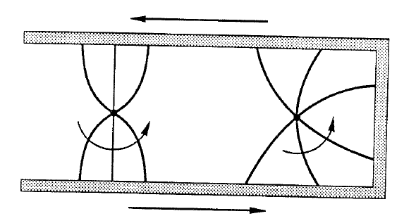
and the Kelvin wave ‘turns the corner’. This suggests that in a long thin basin, one free mode is obtained simply by having an integral number of Kelvin wavelengths around the circumference. However, all of the foregoing assumes basins with flat bottoms and perpendicular walls at the edges. Bottom topography and/or sloping edges introduce yet other modes. The problem of finding the seiches of a rotating basin is not solvable in closed form for most basins because the boundary condition \(\vec u\cdot\hat n=0\) does not admit separable solutions.
Despite these difficulties, the above ideas have been applied to the problem of ocean tides, particularly in long thin marginal seas (e.g. Hendershott and Speranza, 1971). Two such basins are the Adriatic Sea and the Gulf of California. In the Adriatic Sea, the \(M_2\) tide has a typical cotidal form which has been known since the beginning of the century. Hendershott modelled the \(M_2\) tide with two Kelvin waves travelling in opposite directions along the basin meridional coastlines. To close the problem at the Northern border, Hendershott allowed for an infinite series of Poincaré waves just as described above. The Gulf of California is similar to the Adriatic Sea in shape and bottom topography. However, the Gulf of California has no amphidromic point! Why? The difference is due to bottom friction. In the Adriatic Sea, the bottom friction is small, so the reflected Kelvin wave at the northern boundary has an amplitude nearly equal to the incident Kelvin wave. This allows the existence of an amphidromic point. The bottom friction in the Gulf of California is much larger due to the shallow, broad shelf at the northern end. The effect is to damp out the reflected
Kelvin wave so that its amplitude is much smaller than the incident amplitude. When these two waves are superimposed, the amphidromic point is shifted toward the side with the reflected Kelvin wave (west in this case). If the bottom friction is strong enough, the amphidromic point will be located outside the basin, becoming a virtual amphidromic point.
Rossby and planetary waves
These waves were first discovered by Hough (1897, 1898) who solved LTE on a spherical earth for a shallow ocean by expanding the solution in powers of \(\sin\theta\). He found two classes of solutions. The first corresponds to the long gravity waves modified by rotation (Sverdrup waves) which we have already seen. The second class of solutions was found when the second order term in the expansion, \(\sin^2\theta\), was retained. That is, these waves appeared when the variation of rotation with latitude was allowed. In 1939, Rossby rediscovered Hough’s second class of solutions by allowing the rotation rate to vary with latitude, but in Cartesian coordinates. This means that he considered the so-called \(\beta\)-plane approximation (rather than the \(f\)-plane) in which the Coriolis parameter varies linearly in the north-south direction \[f=f_0+\beta y.\] Otherwise, the equations of motion remain the same. Also, we typically treat \(f\) as a constant everywhere except where it is differentiated with respect to \(y\).
Before launching into the new wave types, consider momentarily the shallow water equations with variable depth \[u_t-fv=-g\eta_x \ ;\qquad v_t+fu=-g\eta_y.\]
\[\eta_t+(uD)_x+(vD)_y=0.\] We can form a vorticity equation by differentiating the \(x\) momentum equation with respect to \(y\) and subtracting this from the derivative of the \(y\) momentum equation with respect to \(x\). \[(v_x-u_y)_t=-\beta v+\frac{f}{D}\vec u\cdot\nabla D+\frac{f}{D}\eta_t.\] Take, for example, \(D=e^{-By/f}\), i.e. depth decreasing toward the north. Then the vorticity equation becomes \[(v_x-u_y)_t=-\beta v-Bv+\frac{f}{D}\eta_t.\] This immediately shows that a variable relief which decreases toward the north has the same dynamical effect on the motion as the variation of rotation with latitude. Thus, the type of planetary motions we shall now study will have an analogous counterpart in the absence of \(\beta\) but with \(y\)-dependent relief. Furthermore, if the topography varies in a different direction so as to dominate the \(\beta v\) effects, then the following discussions could be applied to that situation (with minor modifications) by defining a new ‘effective northward’ direction. This is an important idea to which we will return later.
We first consider the problem solved by Rossby of motion in a shallow, horizontally nondivergent ocean. \[\begin{aligned} u_t-fv & =-g\eta_x, & v_t+fu & =-g\eta_y, \\ u_x+v_y & =0. \end{aligned}\] The vorticity equation is \[(v_x-u_y)_t+\beta v=0.\]
(5.15)
The local rate of change of the relative vorticity balances the change in planetary vorticity. Since the flow is nondivergent, we can introduce a streamfunction \[u=-\psi_y \ ;\qquad v=\psi_x.\]
and we obtain \[\nabla^2\psi_t+\beta\psi_x=0.\] This has a plane wave solution of \[\psi=e^{-i\sigma t+ikx+i\ell y}\] with the dispersion relation \[\sigma=-\frac{\beta k}{k^2+\ell^2}.\]
(5.16)
This can be rewritten as \[\left(k+\frac{\beta}{2\sigma}\right)^2+\ell^2 =\left(\frac{\beta}{2\sigma}\right)^2\] which is easy to plot on the \((k,\ell)\) plane.
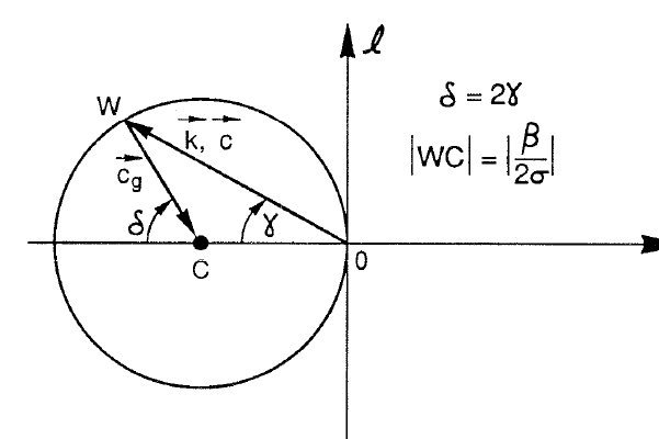
The allowed loci of wavenumbers \((k,\ell)\) form circles in the \((k,\ell)\) plane with the center at \((-\beta/2\sigma,0)\) and with radius \(\beta/2\sigma\). If \(\ell=0\), then \(\sigma=-\beta/k\) and \(c=\sigma/k=-\beta/k^2\). The phase speed \(c\) always has a westward component for whatever value of \(\ell\) we choose. In general \[c_x=\frac{\sigma}{k}=-\frac{\beta}{k^2+\ell^2}, \qquad c_y=\frac{\sigma}{\ell} =-\frac{\beta k}{\ell(k^2+\ell^2)}.\] These waves are called Rossby waves.
The physical mechanism which makes Rossby waves propagate westward is most easily seen for nearly zonal waves \(\partial/\partial y\ll\partial/\partial x\). Then the vorticity equation is simply \[(v_x)_t+\beta v=0.\] North-south motions \(v\) result in changes in the local vorticity. When the north-south motion is periodic in \(x\), then the additional north-south motion generated by the vorticity resulting from the initial pattern combines with this pattern to shift it westward.
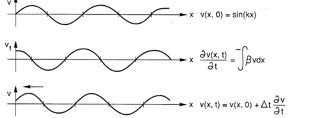
The group velocity components are \[\begin{aligned} c_{gx}=\frac{\partial\sigma}{\partial k} & =-\frac{\beta}{K^2}+\frac{2\beta k^2}{K^4} =\frac{\beta(-K^2\sin^2\gamma+K^2\cos^2\gamma)}{K^4} =\frac{\beta\cos(2\gamma)}{K^2}, \\ c_{gy}=\frac{\partial\sigma}{\partial\ell} & =\frac{2\beta k\ell}{K^4} =-\frac{\beta\sin(2\gamma)}{K^2}, \end{aligned}\] so the total group velocity vector is \[\vec c_g=\frac{\beta}{K^2} [\hat i\cos(2\gamma)-\hat j\sin(2\gamma)].\]
(5.17)
The situation is as depicted in the dispersion diagram. That is, \[\vec c_g =\frac{2\sigma}{K^2}|WC|[\hat i\cos\delta-\hat j\sin\delta] =\frac{2\sigma}{K^2}\overrightarrow{WC'}\]
directed along \(WC'\) towards \(C'\). We then have an easy way to visualize the flow of energy and phase. A westward going wave transmits energy eastward. As the phase propagates more northwest, energy propagates more southeast.
It is interesting to note that, for these nondivergent waves, the velocity vector is normal to the wavenumber. This can be easily seen from continuity, since \(u_x+v_y=0\) which, for a plane wave solution, can be written \[(ik\hat i+i\ell\hat j)\cdot\vec u=0.\] Thus, in a westward propagating wave, \[v=\psi_x=ik\psi, \qquad u=-\psi_y=-i\ell\psi=0.\] This is quite different from the usual case of nonrotating, divergent gravity waves.
A second type of planetary wave was first studied by Bjerknes (1937). In this case, the horizontal accelerations are negligible, but the flow is divergent. Thus, we allow for a surface elevation in continuity, but the horizontal velocities are in geostrophic balance. \[-fv=-g\eta_x, \qquad fu=-g\eta_y,\] \[\eta_t+D(u_x+v_y)=0.\] Combining these into a single equation yields \[\eta_t-\frac{g\beta D}{f^2}\eta_x=0.\] This is a simple first order wave equation which has the general solution \[\eta=F\left(x+\frac{g\beta D}{f^2}t\right)\] where \(F\) is any function. Thus, a sea-surface elevation of any shape will propagate unaltered in this dynamical system. Looking for a plane wave solution of the form \[\eta=e^{-i\sigma t+ikx+i\ell y}\] we find the dispersion relation \[\sigma=-\frac{g\beta D}{f^2}k.\]
(5.18)
The phase speed is again westward \[c=-g\beta D/f^2\] and the group velocity is \[\vec c_g=\hat i c_{gx}=\hat i\frac{\partial\sigma}{\partial k} =-\frac{g\beta D}{f^2}\hat i.\] These waves are divergent, nondispersive planetary waves in contrast to the previous Rossby waves which are nondivergent but dispersive. The north-south wavenumber is arbitrary and the dispersion relation on the \((k,\ell)\) plane is
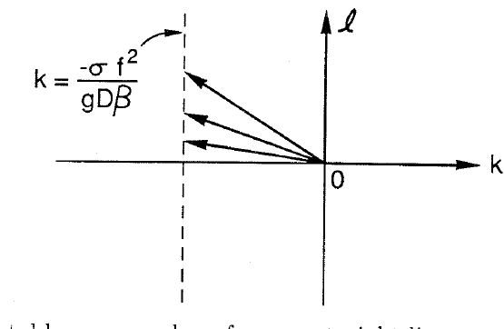
The locus of acceptable wavenumbers forms a straight line.
The physical mechanism which causes these waves to propagate westward is now very different from that for Rossby waves. Remember that the flow is totally geostrophic but divergent. Consider a region of high pressure
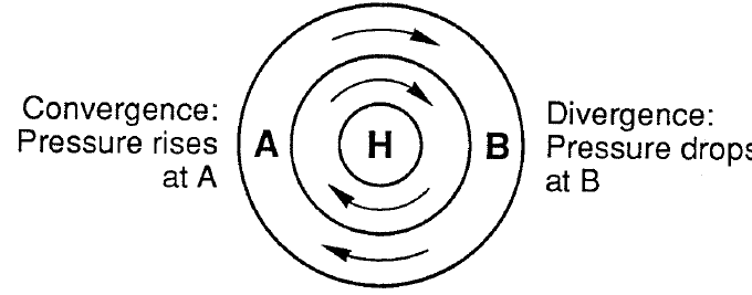
The flow at A converges because the transport (geostrophic) between a pair of isobars south of \(H\) is greater than that between the same pair north of \(H\) because \(f\) varies. By continuity, pressure must rise at A. Similarly, the flow at B diverges and the pressure
there drops. The initial pattern of isobars is then shifted westward and the pressure high moves toward A. The same is true for a pressure low as you can verify for yourselves.
Now consider the general system of which the two previous wave types were limiting cases. \[\begin{aligned} u_t-fv & =-g\eta_x, & v_t+fu & =-g\eta_y, \\ \eta_t+D(u_x+v_y) & =0. \end{aligned}\] In the usual way, we assume time dependence of \(e^{-i\sigma t}\) and combine the equations to form a single equation for \(v\) in this case. \[\nabla^2v+\frac{i\beta}{\sigma}v_x +\frac{\sigma^2-f^2}{gD}v=0.\] Notice that the first two terms are the same as those in the nondivergent Rossby wave balance. Now \(f\) is not really constant, but we consider it fixed in order to look for plane wave solutions \(v=e^{ikx+i\ell y}\). The dispersion relation is \[\left(k+\frac{\beta}{2\sigma}\right)^2+\ell^2 =\left(\frac{\beta}{2\sigma}\right)^2 +\frac{\sigma^2-f^2}{gD}\]
(5.19)
which can be drawn on the \((k,\ell)\) plane as
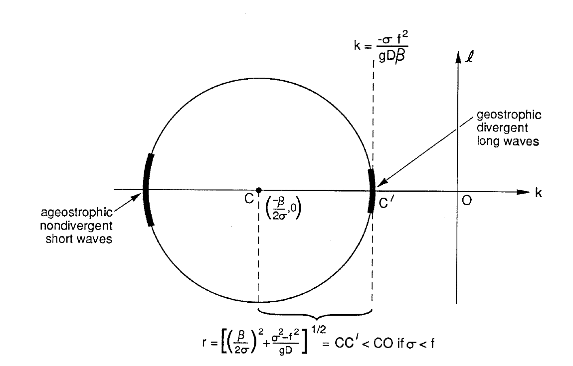
Notice the following limits
a) \(\sigma\ll f\) and \(k,\ell\) small. The dispersion relation becomes \[\beta k/\sigma+f^2/gD\simeq0 \quad\Rightarrow\quad \sigma=-\frac{g\beta D}{f^2}k.\] This is the limit of geostrophic, divergent long waves.
b) \(\sigma\ll f\) and \(k\) large, \(\ell\) arbitrary. The dispersion relation becomes \[(k^2+\ell^2)+\beta k/\sigma\simeq0 \quad\Rightarrow\quad \sigma=-\frac{\beta k}{k^2+\ell^2}.\] This is the limit of ageostrophic, nondivergent short Rossby waves.
Notice that for the waves to exist, the radius of the circle must be positive \[\left(\frac{\beta}{2\sigma}\right)^2 +\frac{\sigma^2-f^2}{gD}>0.\] In the Rossby wave limit \(\sigma\ll f\), the above relationship is \[\sigma<\frac{\beta(gD)^{1/2}}{2f}\simeq0.2f\] that is, \[T>\frac{4\pi f}{\beta(gD)^{1/2}}.\]
which is about 3 days for a barotropic wave (\(\beta=2.3\times10^{-11}\ \mathrm{m^{-1}\,s^{-1}}\)) but many days for a baroclinic wave with \(D=d_n\), the equivalent depth. If instead we let \(\sigma\to\infty\), we obtain \[\sigma^2=f^2+gD(k^2+\ell^2)\] which is simply the shallow water gravity waves modified by rotation, with \(\sigma\gg f\). The following sketch shows the two dispersion relations together, for the first and second class waves.
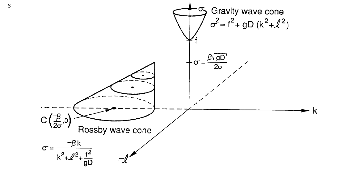
The top of the Rossby wave cone is defined by \(r=0\) which occurs at a small fraction of \(f\), so there is a frequency interval between \(f\) and \(\beta(gd_n)^{1/2}/2f\) separating the two classes of solutions. This gap suggests that velocity spectra should show a valley between these two frequencies with a high frequency boundary at \(f\) and a low frequency boundary at \(\beta(gd_n)^{1/2}/2f\). Such an energy gap is indeed observed, but remember that the linearized dynamics on the \(\beta\)-plane are very simplified and the dynamics of the low frequency motions may need a more complete treatment.
The dispersion relation is usually written (for \(\sigma\ll f\)) as \[\sigma=-\frac{\beta k} {k^2+\ell^2+f^2/gD}.\]
(5.20)
The length scale \[a_r=(gD)^{1/2}/f\] is called the Rossby radius. There is not one Rossby radius, but an infinite number because of the infinite sequence of internal modes, each with a different equivalent depth and, therefore, a baroclinic Rossby radius. Waves which are longer than the Rossby radius are long, divergent Rossby waves. Waves that are shorter than the Rossby radius are short, nondivergent Rossby waves. The barotropic Rossby radius has \(D\sim d_0\) (ocean depth) and is thus of the order of the earth’s radius. Barotropic Rossby waves are therefore, relatively high frequency (typically a few cycles per month) and are able to traverse major ocean basins in days to weeks. Baroclinic Rossby radii are of the order of 100 km or less in mid-latitudes, and the baroclinic Rossby waves are relatively low frequency waves. It would take them years to cross ocean basins. Notice, however, that going towards the equator \(f\to0\) and the baroclinic Rossby waves speed up to the point where they could traverse major ocean basins in a season. But then we must relax the mid-latitude \(\beta\)-plane dynamics and study the problem with the appropriate equatorial dynamics (which we will do shortly).
Rossby wave reflection
Consider the reflection of a Rossby wave from a straight wall making some arbitrary angle \(\mu\) with the \(x\) axis.
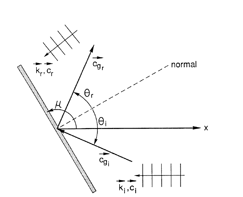
If there is a reflected wave, then both incident and reflected waves must have the same wavenumber component along the wall. This can be seen by considering the case of \(\mu=90^\circ\). (The computation can be done for any wall angle by choosing coordinates parallel and perpendicular to the wall.) The incident wave is \[\psi_i=A_i e^{i(k_i x+\ell_i y-\sigma_i t)}\] while the reflected wave is \[\psi_r=A_r e^{i(k_r x+\ell_r y-\sigma_r t)}.\] At \(x=0\) the total streamfunction \((\psi_i+\psi_r)\) must be constant so that \(u=-\partial\psi/\partial y=0\). Without loss of generality, we can take the constant to be zero. Thus \[A_i e^{i(\ell_i y-\sigma_i t)} +A_r e^{i(\ell_r y-\sigma_r t)}=0.\] For this to be true for all time and for all \(y\), then \(\sigma_i=\sigma_r=\sigma\) and \(\ell_i=\ell_r=\ell\).
We can use the sketch of the dispersion relation to visualize the reflection properties.
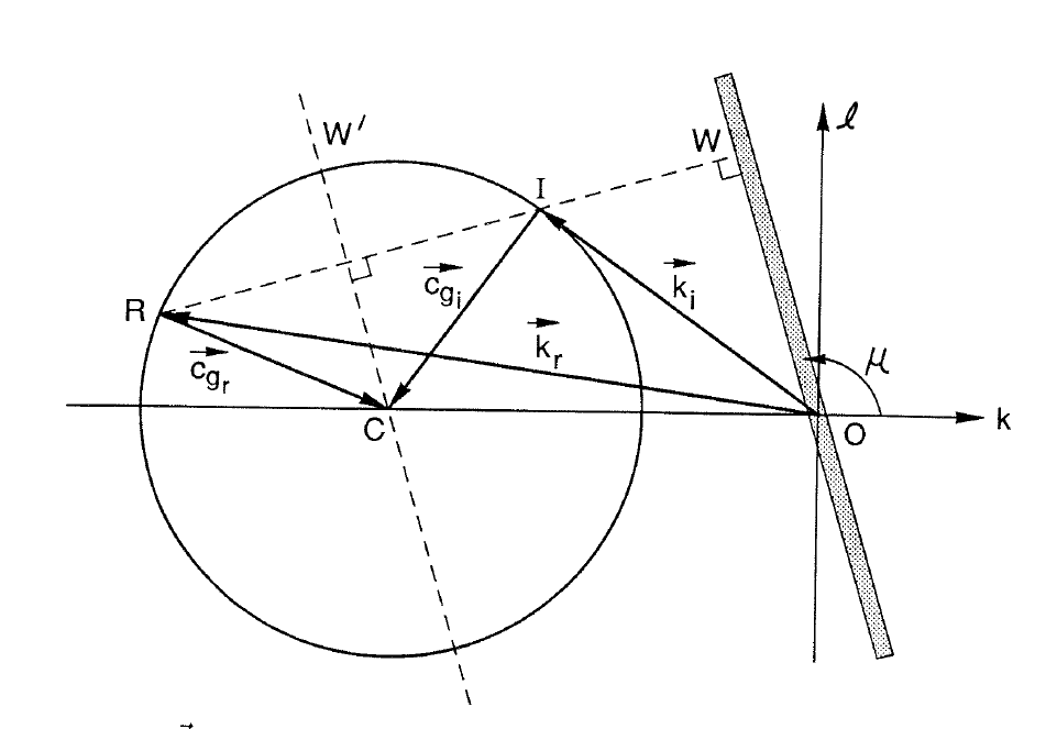
The projection of \(\vec k_i\) on the wall must equal the projection of \(\vec k_r\). This fixes the point \(R\) for the reflected \(\vec k_r\). Construct the line \(CW'\) parallel to \(OW\). Then angle \(ICW'\) equals angle \(W'C'R\), that is the group velocity (and consequently the energy flux) of the incident wave is reflected with the same angle to the wall. From the streamfunction argument, it also follows that \[A_i=-A_r=A.\] The amplitude of the reflected wave is equal to the amplitude of the incident wave with a phase shift of \(180^\circ\). Because the reflection is specular for the group velocity and energy flux, the components of the energy flux normal to the wall are equal and opposite. From the dispersion relation, knowing \(\sigma\) and \(\ell\), we can solve for \(k\). There are two roots and only one is appropriate to energy going towards the wall: that gives \(k_i\). The other solution must give \(k_r\). The change in \(k\) due to reflection is (we are in the limit \(\sigma\ll f\) for which \(\sigma^2\) is neglected compared to \(f^2\)) \[k_r-k_i=-2\left[ \frac{\beta^2}{4\sigma^2} -\left(\ell^2+\frac{f^2}{gD}\right) \right]^{1/2}.\] Thus, we see that the long waves are reflected as shorter waves from a western boundary while short waves are reflected as longer ones from an eastern boundary. To
see this remarkable property of Rossby waves better, consider the following two limiting cases.
a) Wave with \(\ell=0\), propagating energy westward and reflected at a western wall
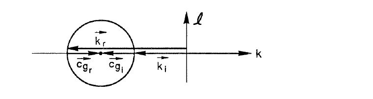
This will be reflected as a much shorter wave propagating energy eastward.
b) Wave with \(\ell=0\), propagating energy eastward and reflected from an eastern wall.
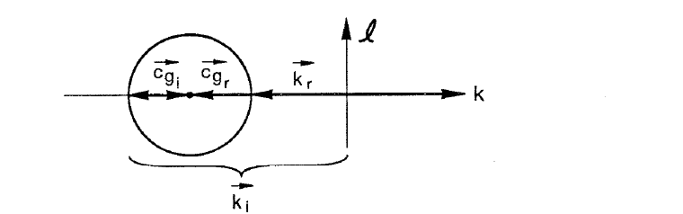
This will be reflected by the eastern wall as a longer wave propagating energy westward. Thus, if we generate waves of equal wavelengths in the middle of the ocean moving east and west, we will get short waves back from the west and long waves back from the east.
Western boundary current formation
We now discuss briefly the interpretation of the formation of a western boundary current based on Rossby wave ideas which was originally put forth by Pedlosky. Each of the dynamically different steady circulation models of the ocean general circulation share the common feature of westward intensification despite other noticeable differences. A simple physical explanation can be found considering time dependent
dynamics and the character of Rossby waves. As we have seen, energy in the short waves will be transmitted eastward while energy in the long waves will propagate westward. Suppose that at some time, energy of varying length scales is input to the ocean by the wind stress. The small scale components will move to the eastern boundary where they will be reflected as long wave components, with waves extending into the gyre interior. On the other side, the long scale components will propagate energy toward the western boundary where they will be reflected as short scale motions. The western boundary thus acts as a source of energy in the short scales, concentrated in a width of the order of the western boundary layer. (See Pedlosky, 1979, pp. 278–281 for more details.)
Equatorial waves
All of the planetary waves which we have studied are valid on a mid-latitude \(\beta\)-plane in which the variation in rotation is small compared to the basic rotation, i.e. \(\beta y<f_0\). The dynamics change considerably if we go to the equatorial region where \(f_0\to0\). Then we can approximate \(f\) by \(\beta y\) and ignore \(f_0\). The equations of motion become \[\begin{aligned}u_t-\beta yv&=-g\eta_x, &v_t+\beta yu&=-g\eta_y,\\ \eta_t+D(u_x+v_y)&=0.\end{aligned}\]
(5.21)
This is called the equatorial \(\beta\)-plane because we have approximated the sphere by a plane tangent to the equator. If we assume time dependence of \(e^{-i\sigma t}\) and solve for \(v\) as we did for the mid-latitude planetary waves, we obtain \[\nabla^2v+\frac{i\beta}{\sigma}v_x +\left(\frac{\sigma^2-\beta^2y^2}{gD}\right)v=0.\]
This equation does not have constant coefficients, so we cannot assume a plane wave solution. Instead, we take a plane wave only in the east-west (\(x\)) direction \[v=v(y)e^{ikx}.\] The equation for \(v\) becomes \[v_{yy}+\left( \frac{\sigma^2}{gD}-k^2-\frac{\beta k}{\sigma} -\frac{\beta^2y^2}{gD} \right)v=0\] with boundary conditions of \[\lim_{y\to\pm\infty}v=0\] to preserve internal consistency in the equatorial approximation, since we cannot move to regions where \(f_0\) becomes large.
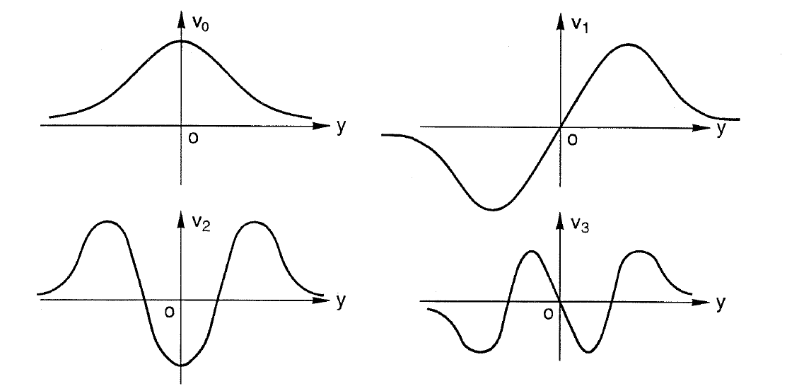
The equation for \(v\) looks very much like Hermite’s equation \[\psi_{\xi\xi}+(\kappa-\xi^2)\psi=0 \qquad\text{with}\qquad \kappa=2m+1,\quad m=0,1,2,\ldots\] We make the change of variables \[y=\xi(gD)^{1/4}/\beta^{1/2}\] and we obtain \[v_{\xi\xi}+\left[ \frac{(gD)^{1/2}}{\beta} \left(\frac{\sigma^2}{gD}-k^2-\frac{\beta k}{\sigma}\right) -\xi^2 \right]v=0.\] The solutions are \[v_m=e^{-\beta y^2/[2(gD)^{1/2}]} H_m\!\left[\beta^{1/2}y/(gD)^{1/4}\right]\] with a dispersion relation of \[\frac{(gD)^{1/2}}{\beta} \left(\frac{\sigma^2}{gD}-k^2-\frac{\beta k}{\sigma}\right) =2m+1.\]
(5.22)
The \(H_m\) are the Hermite polynomials \[H_0=1;\qquad H_1=2\xi;\qquad H_2=-2+4\xi^2\ldots\]
and the solution decays exponentially as \(y\to\pm\infty\) as we required. Thus, various \(v_m\) look like
To explore the possible wave solutions, we make the following transformations \[\sigma=\omega\beta^{1/2}(gD)^{1/4}; \qquad k=\lambda\beta^{1/2}/(gD)^{1/4}\] where \(\omega\) is the dimensionless frequency and \(\lambda\) is the dimensionless east-west wavenumber. The dispersion relation becomes \[\omega^2-\lambda^2-\lambda/\omega=2m+1.\]
(5.23)
This is a cubic in \(\omega\). For given wavenumbers \(m\) and \(k\), three frequencies are generally specified. To see their connection with previous work, consider the following limiting cases.
a) Limit of short waves \(\lambda\to\pm\infty\) with high frequency \(\omega\to\infty\). Then \(\lambda/\omega\) is constant and the dispersion relation is \[\omega^2=\lambda^2+2m+1\]
which asymptotically tends to \(\omega=\pm\lambda\). In dimensional form, the two asymptotes correspond to \[\sigma=\pm(gD)^{1/2}k.\] These are high-frequency, short, shallow water gravity waves which exist for \(\sigma\to\infty\). They are trapped at the equator and move eastward and westward.
b) Limit of short waves \(\lambda\to\pm\infty\) with low frequency \(\omega\to0\). The dispersion relation becomes \[\omega=-1/\lambda\] which, in dimensional form, is \[\sigma=-\beta/k.\] This is the Rossby wave limiting case of the dispersion relation for short planetary waves which are trapped at the equator and move energy eastward.
c) Limit of long waves \(\lambda\to0\) with low frequency \(\omega\to0\). The dispersion relation becomes \[\omega=-\frac{\lambda}{2m+1}\] which, in dimensional form, is \[\sigma=-\frac{(gD)^{1/2}k}{2m+1}.\] These are Rossby wave modes with long wavelengths which asymptotically approach the previous Rossby wave limiting case as the wavelength decreases. The above cases are the limiting forms of the three roots for \(m\ge1\) which exist for the general dispersion relation. The solutions are two oppositely travelling shallow water gravity waves plus a westward (phase) planetary wave solution.
d) For the case \(m=0\), we have the Yanai or mixed gravity-Rossby wave solution. We can write the dispersion relation as \[(\lambda+\omega)[\lambda-(\omega-1/\omega)]=0.\]
(5.24)
Note that \(\omega=-\lambda\) does not solve the original momentum equations, so we must take \[\lambda=\omega-1/\omega\] which, in dimensional form, is \[k=\frac{\sigma}{(gD)^{1/2}}-\frac{\beta}{\sigma}.\] If \(\sigma\to0\), then \(\sigma\simeq-\beta/k\) and we have the Rossby wave properties dominating. If \(\sigma\to\infty\), then \(\sigma=(gD)^{1/2}k\) and we have the gravity wave properties dominating. Thus, the Yanai wave is of gravity type when propagating (phase) eastward and of planetary type when propagating westward.
e) The case \(m=-1\) is an equatorially trapped Kelvin wave. In fact, the solution to the original system can be found when \(v=0\) everywhere or by deriving an equation for \(u\) rather than \(v\) and solving it. The equations are \[\begin{aligned} i\sigma u & =g\eta_x, & \beta yu & =-g\eta_y, \\ -i\sigma\eta+Du_x & =0. \end{aligned}\] The physical balance in the momentum equations is geostrophic in the north-south direction and local acceleration versus pressure gradient in the east-west direction. These are the balances typical of Kelvin waves. Assuming the plane wave form in \(x\), i.e. \(e^{ikx}\), we find a solution of the form \[\eta=e^{-\beta k y^2/(2\sigma)}e^{-i\sigma t+ikx}.\] Notice that these waves exist only if \(k>0\) to satisfy the requirement of decaying away from the equator. They are trapped at the equator and move only eastward. Substituting the solution into the continuity equation gives a dispersion relation of \[\sigma=(gD)^{1/2}k.\]
(5.25)
which is simply the gravity wave dispersion relation which we also found for Kelvin waves on an \(f\)-plane. In a configuration with north-south boundaries, these eastward propagating Kelvin waves, trapped at the equator, can close the circulation as shown in the following sketch.
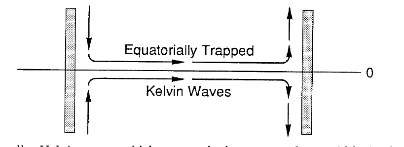
Thus, conceptually, Kelvin waves which approach the equator from mid-latitudes become equatorially trapped Kelvin waves which propagate to the eastern boundary. There they change again to mid-latitude Kelvin waves propagating northward along the boundary.
We can summarize all the equatorially trapped wave solutions in the following dispersion diagram.
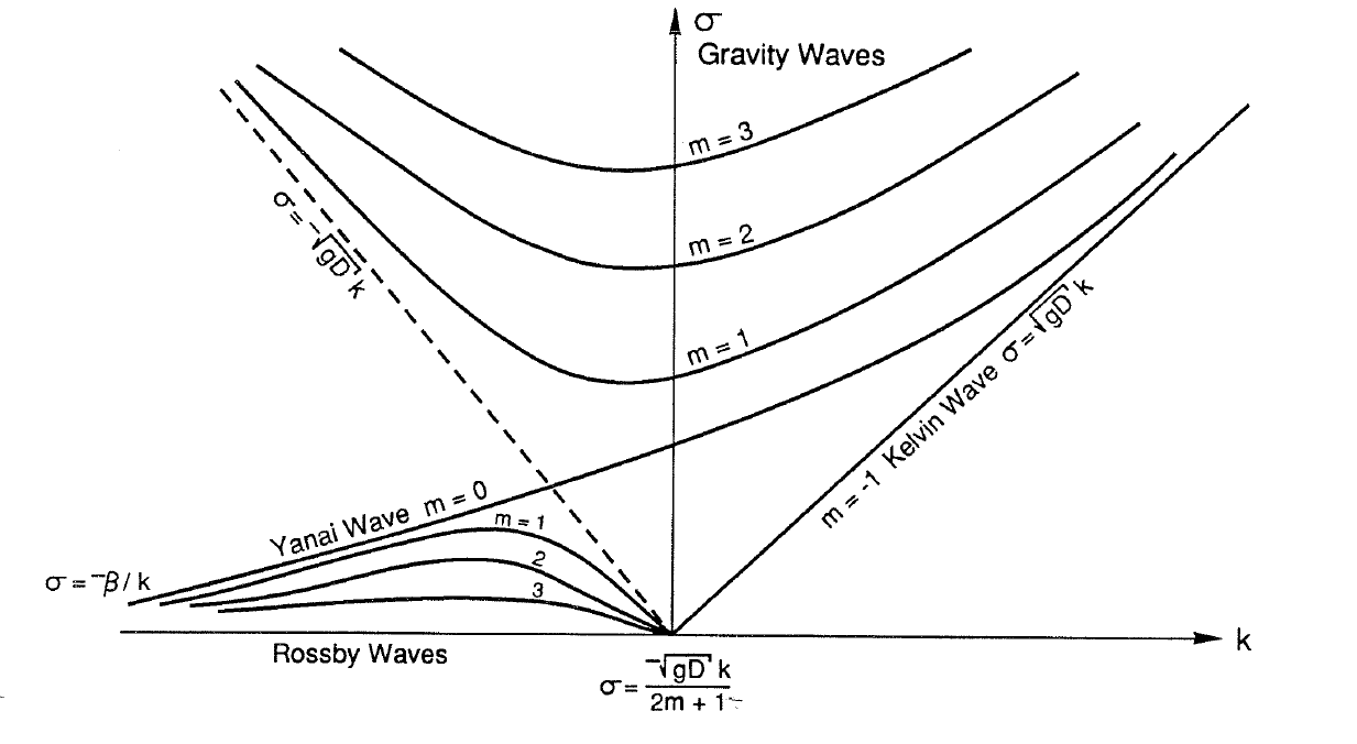
We know that trapping means that a wave decays exponentially away from some boundary. We have seen that this corresponds to the total reflection of wave rays as well. Therefore, it is useful to examine these equatorial waves with the ray method which we discussed earlier in the course. We force a plane wave solution to satisfy the equation for \(v\) \[v=v_0(y)e^{-i\sigma t+ikx+i\ell(y)y}.\] Then the dispersion relation becomes (provided \(v_0\) varies slowly so that \(v_{0yy}\) is always small) \[\ell^2(y)=\frac{\sigma^2}{gD}-k^2-\frac{\beta k}{\sigma} -\frac{\beta^2y^2}{gD}.\]
(5.26)
Now the ray path is defined by \[\frac{dy}{dx}=\frac{\ell}{k} =\left( \frac{\sigma^2}{gDk^2}-1-\frac{\beta}{\sigma k} -\frac{\beta^2y^2}{gDk^2} \right)^{1/2}.\] We can define the angle that the ray makes at the equator (\(y=0\)) by \[\tan\theta_0=\frac{\ell(0)}{k} =\left( \frac{\sigma^2}{gDk^2}-1-\frac{\beta}{\sigma k} \right)^{1/2}.\] Then, we can integrate along the ray path by using \[\int\frac{dy}{(a^2-b^2y^2)^{1/2}} =\int dx \quad\Rightarrow\quad \frac{1}{b}\sin^{-1}\frac{by}{a}=x+\mathrm{const}\] to find \[y=\frac{(gD)^{1/2}k}{\beta}\tan\theta_0 \sin\left( \frac{\beta}{(gD)^{1/2}k}x+\mathrm{const} \right).\] This says that rays are sinusoids moving around the equator
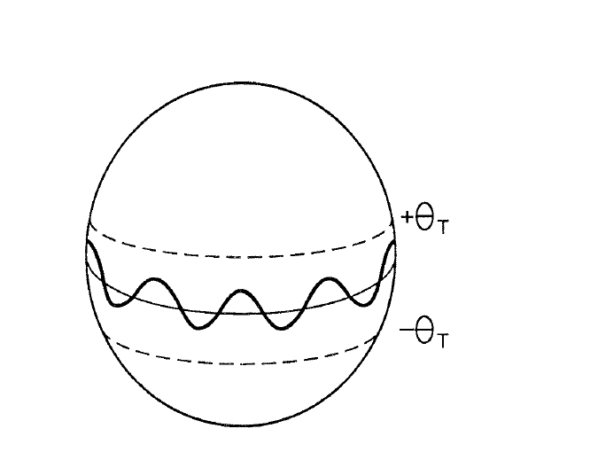
They go back and forth between the two latitudes \(\pm\theta_T\), being continuously refracted by the varying \(f=\beta y\), which models the curvature of the earth.
We can find the trapping latitudes \(\pm\theta_T\) where the rays are totally reflected. They are simply the maxima of \(y\) \[\pm\theta_T=\pm\frac{(gD)^{1/2}k}{\beta}\tan\theta_0.\]
(5.27)
If \(k\to0\), that is the waves squash together propagating only north and south, then the ray path degenerates into the straight line \[-\sigma/\beta\le y\le\sigma/\beta\] which says that, since \(\sigma=\pm\beta y=\pm f\), the waves must remain within their inertial latitudes. There the rays must turn back toward the equator. If \(k\ne0\), then the turning latitude moves equatorward, at least when \(k/\sigma\) is not important. The inertial latitudes thus act as a natural waveguide for waves of a given frequency. Poleward of the inertial latitudes, gravity waves cannot propagate. Equatorward, they may. It is important to remember that the inertial latitudes are not solid barriers, however. The wave structure decays exponentially poleward with a scale which is determined by the particular wave. Furthermore, the decay scale is very different for the barotropic waves versus their baroclinic counterparts. An analysis of the Hermite functions shows that
the barotropic wave decays on a scale of the order of the earth’s radius, thus violating our original assumption of the \(\beta\)-plane. The baroclinic waves decay much faster, on the order of about 5% of the earth’s radius.