Acoustic waves

Being now equipped with some ideas about wave motions, it is useful to consider an example of waves which occurs in both the ocean and the atmosphere and which can illustrate many of the ideas in a rather simple way. Acoustic or sound waves, as Lighthill (1978) points out, are the most fundamental waves in fluids because they can exist in the absence of any external force field. Instead of gravity or rotation, for example, providing a restoring force for the motions, the restoring force for acoustic waves is the fluid’s resistance to compression (i.e., its compressibility).

Basic physics

When viscous dissipation, rotation and gravitational forces are neglected, the momentum and continuity equations are $$\begin{aligned} \frac{\partial\vec u^{\,*}}{\partial t} +\vec u^{\,*}\cdot\nabla\vec u^{\,*} & =-\frac{1}{\rho^*}\nabla p^*, \\ \frac{\partial\rho^*}{\partial t} +\nabla\cdot(\rho^*\vec u^{\,*}) & =0. \end{aligned}$$

An equation relating density and pressure may be obtained from the first law of thermodynamics (Batchelor, 1967; Chapter 3). It can be shown that, if $\rho^*=\rho^*(p^*,T)$ and the motions are adiabatic so that $\partial S/\partial t=0$ where $S$ is the entropy, then $\rho^*=\rho^*(p^*,S)$ and $$\left(\frac{D\rho^*}{Dt}\right)_S =\left(\frac{\partial\rho^*}{\partial p^*}\right)_S \left(\frac{Dp^*}{Dt}\right)_S.$$ A solution of these equations, although trivial, is $$\rho^*=\rho_0;\qquad p^*=p_0;\qquad \vec u^{\,*}=0.$$ This solution is not very exciting, so we would like to study small deviations from it. Thus, we write $$\rho^*=\rho_0+\rho;\qquad p^*=p_0+p;\qquad \vec u^{\,*}=0+\vec u$$ where $\rho,p,\vec u$ are of infinitesimal amplitude. After substituting into the original equations and neglecting products of small quantities, we have $$\begin{aligned} \frac{\partial\vec u}{\partial t} & =-\frac{1}{\rho_0}\nabla p, \\ \frac{\partial\rho}{\partial t}+\rho_0\nabla\cdot\vec u & =0, \\ \frac{\partial\rho}{\partial t} & =c^{-2}\frac{\partial p}{\partial t}, \end{aligned}$$ where $$c^2=\left(\frac{\partial\rho^*}{\partial p^*}\right)_S^{-1}.$$ After eliminating $\vec u$ and $\rho$ in favor of $p$, we obtain $$\frac{\partial^2p}{\partial t^2}-c^2\nabla^2p=0.$$

We recognize this as a wave equation which was listed in Chapter 1. It is easy to show that the other variables $\rho,u,v,w$ each satisfy a similar equation.

Plane waves

Consider a homogeneous medium; $c(\vec x,t)=c_0$. Then $p=a e^{-i\sigma t+ikx+i{ℓ} y+imz}$ solves the wave equation provided $$\sigma^2=c_0^2(k^2+{ℓ}^2+m^2)$$

which is the dispersion relation. For fixed $\sigma$, the locus of allowed wavenumbers in $k,{ℓ},m$ space is a sphere of radius $\sigma/c_0$. All wavenumbers $\vec k=k\hat i+{ℓ}\hat j+m\hat k$ extending from the center of this sphere to its surface are allowed. In a given plane wave, phases propagate along the wavenumber vector at speed $c_0$; that is, $\sigma/|\vec k|=c_0$, so the waves are nondispersive. The group velocity $\vec c_g$ is defined by $$c_{gx}=\frac{\partial\sigma}{\partial k};\qquad c_{gy}=\frac{\partial\sigma}{\partial{ℓ}};\qquad c_{gz}=\frac{\partial\sigma}{\partial m}$$ and it is easy to show that $|\vec c_g|=c_0$.

If $p=a e^{i(\vec k\cdot\vec x-\sigma t)}$, then the momentum equations say $-i\sigma\vec u=-i\vec k p/\rho_0$, or $$\vec u=\frac{\vec k a}{\sigma\rho_0} e^{i(\vec k\cdot\vec x-\sigma t)}.$$ This means that $\vec u$ and $\vec k$ are parallel, i.e. these are longitudinal waves (displacement is parallel to the direction of wave propagation). Also, $\vec u$ and $p$ are in phase in this travelling plane wave.

Reflection at a solid boundary

Suppose a plane wave of the form $$p_{inc}=p_0e^{-i\sigma t+ikx+i{ℓ} y-imz}$$

is incident upon a solid boundary. At the solid boundary, the normal velocity must vanish; $\vec u\cdot\hat n=0$ which means that $\nabla p\cdot\hat n=0$. If the solid boundary is at $z=0$, then the boundary condition is $$p_z=0\qquad\text{at }z=0.$$

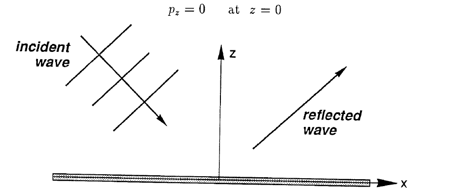
To satisfy this boundary condition, we must add a reflected wave $$p_{ref}=p_0e^{-i\sigma t+ikx+i{ℓ} y+imz}$$ to the incident wave. The solution is $$p=p_{inc}+p_{ref}=2p_0e^{-i\sigma t+ikx+i{ℓ} y}\cos mz.$$

Suppose the solid boundary is tilted, say $z=\alpha x$, and the incident energy approaches along $\vec k_i$ while the reflected energy travels along $\vec k_r$.

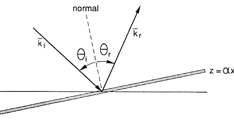
If $p_{inc}$ and $p_{ref}$ are to sum such that $p=p_{inc}+p_{ref}$ satisfies $\partial p/\partial n=0$ at the solid boundary, then we must have $$|\vec k_i|\cos\theta_i=|\vec k_r|\cos\theta_r,$$ i.e., the projection of the incident wavenumber on the boundary must equal the projection of the reflected wavenumber on the boundary. But we know that $|\vec k_i|=|\vec k_r|=\sigma/c_0$, so $\theta_r=\theta_i$. That is, the reflection of these waves is specular. (This is not true of all waves, however.) Note that $\partial p/\partial n=0$ at the boundary means $\vec u\cdot\hat n=0$ there, so $\vec u_{inc}\cdot\hat n=-\vec u_{ref}\cdot\hat n$.

Plane waves in a channel

A very important aspect of wave motion is the effect of boundaries which form a channel or waveguide. Thus far, the plane waves we have considered have not been restricted in the choice of wavenumbers. That is, the entire continuum of $k,{ℓ},m$ choices has been available, provided we were willing to accept whatever frequency was required by the dispersion relation. We saw that the form of the plane wave was altered somewhat due to the presence of one boundary, so now we consider the effect of a second boundary.

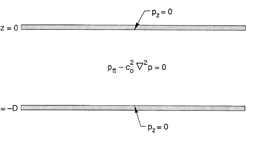
Now the field equation is still valid in the interior of the channel, but the free waves must satisfy $\partial p/\partial z=0$ on both boundaries, at $z=0,-D$. To find a solution, we assume that the waves are free to travel along the channel, but that the cross-channel dependence is unknown. $$p(x,y,z,t)=p_0e^{-i\sigma t+ikx+i{ℓ} y}P(z).$$ This is substituted into the field equation to obtain an equation for the cross-channel structure $$P_{zz}+(\sigma^2/c_0^2-k^2-{ℓ}^2)P=0$$ $$P_z=0\qquad\text{at }z=0,-D.$$ This equation has the solution $$P(z)=\cos n\pi z/D$$ provided that $$\sigma^2/c_0^2=k^2+{ℓ}^2+n^2\pi^2/D^2, \qquad n=0,1,2,\ldots$$

Notice that these solutions are each a sum of two plane waves $$\frac12p_0e^{-i\sigma t+ikx+i{ℓ} y+in\pi z/D} +\frac12p_0e^{-i\sigma t+ikx+i{ℓ} y-in\pi z/D}$$ which satisfy $\partial p/\partial z=0$ at $z=0$ regardless of whether $n$ is an integer or not. However, to satisfy $\partial p/\partial z=0$ at $z=-D$, we need $n=0,1,2,\ldots$. These solutions are called waveguide modes.

Another important point to notice is that each three-dimensional plane wave by itself satisfies the dispersion relation, so that both waves are the usual nondispersive plane waves if we think of $n$ as continuously variable. Yet the solution viewed as a two-dimensional plane wave restricted to the channel direction is dispersive! $$c_{ph}=\sigma/(k^2+{ℓ}^2)^{1/2} =\pm c_0\left[1+\frac{n^2\pi^2}{(k^2+{ℓ}^2)D^2}\right]^{1/2}.$$ The horizontal group velocity $\partial\sigma/\partial k$, $\partial\sigma/\partial{ℓ}$ is $$\vec c_g =c_0\frac{k\hat i+{ℓ}\hat j} {(k^2+{ℓ}^2+n^2\pi^2/D^2)^{1/2}}.$$ It is parallel to the horizontal wavenumber $k\hat i+{ℓ}\hat j$ but not equal to the phase velocity.

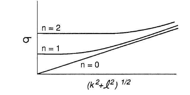
The $n=0$ mode actually is nondispersive.

If we fix the horizontal wavelength $2\pi/(k^2+{ℓ}^2)^{1/2}$, say by a wavemaker of fixed size perhaps but variable frequency, then there is an infinity of waveguide modes

$n=0,1,2,\ldots$ of ever increasing frequency $\sigma^2=c_0^2(k^2+{ℓ}^2+n^2\pi^2/D^2)$. However, if we fix the frequency, then $$(k^2+{ℓ}^2)=\sigma^2/c_0^2-n^2\pi^2/D^2$$ and only for $n=0,1,\ldots n_{max}$ will $k^2+{ℓ}^2>0$ where $n_{max}=\operatorname{int}[(D/\pi)(\sigma/c_0)]$. That is, only for $n=0,1,\ldots n_{max}$ will the waveguide modes propagate down the channel! For example, consider waves in the $x$-direction only $$\begin{aligned} n<n_{max}\qquad p & =e^{-i\sigma t+i(\sigma^2/c_0^2-n^2\pi^2/D^2)^{1/2}x} \cos\frac{n\pi z}{D}, \\ n>n_{max}\qquad p & =e^{-i\sigma t-(n^2\pi^2/D^2-\sigma^2/c_0^2)^{1/2}x} \cos\frac{n\pi z}{D}. \end{aligned}$$ The first set represents travelling waves. The second set represents evanescent waves which decay exponentially away from their source. Practically, this means that if we have a harmonic wavemaker in the channel, then we may expect to see more cross-channel structure near the wavemaker than far away from it.

Scattering at a discontinuity

We have considered the effect of a solid boundary on the propagation of sound waves. Suppose, however, that a plane wave encounters a boundary between two fluids at which the properties change abruptly, i.e. a discontinuity.

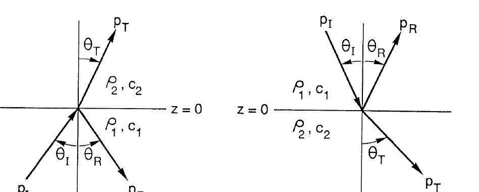
This discontinuity could represent the air-sea interface or the ocean bottom (which is not truly a solid boundary because it transmits sound waves). In both cases the incident wave approaches the discontinuity while travelling through the medium which has density $\rho_1$ and phase speed $c_1$. The density of the medium on the other side is $\rho_2$ while the phase speed is $c_2$.

For the case on the left (upward propagating incident wave), the incident, reflected and transmitted waves have the following forms; $$\begin{aligned} p_I & =a e^{-i\sigma t+ikx+im_1z}, \\ p_R & =Ra e^{-i\sigma t+ikx-im_1z}, \\ p_T & =Ta e^{-i\sigma t+ikx+im_2z}, \end{aligned}$$ where $R$ is the reflection coefficient and $T$ is the transmission coefficient. Notice that the incident and reflected waves have the same wavenumber component in $z$ but that they propagate in opposite directions. The transmitted wave has a different wavenumber in $z$ because the medium has different properties. The wavenumber in the direction of the boundary $x$ as well as the frequency $\sigma$ are the same for all three waves because there is nothing in the fluids which would change them.

To solve the problem, we require that the pressure as well as the velocity normal to the boundary $w$ be continuous across the boundary. That is $$\begin{aligned} p_I+p_R & =p_T & & \text{at }z=0, \\ \frac{1}{\rho_1}(p_{Iz}+p_{Rz}) & =\frac{1}{\rho_2}p_{Tz} & & \text{at }z=0. \end{aligned}$$ Now, substituting the expressions for $p_I,p_R$ and $p_T$, we obtain $$\begin{aligned} 1+R & =T, \\ \frac{m_1}{\rho_1}(1-R) & =\frac{m_2}{\rho_2}T. \end{aligned}$$ From the dispersion relation, $m=\sigma\cos\theta/c$ which changes the second matching condition to $$\frac{1}{\rho_1c_1}(1-R)\cos\theta_I =\frac{1}{\rho_2c_2}T\cos\theta_T.$$ These can be combined to yield $$R=\frac{\rho_2c_2\cos\theta_I-\rho_1c_1\cos\theta_T} {\rho_2c_2\cos\theta_I+\rho_1c_1\cos\theta_T}$$

$$T=\frac{2\rho_2c_2\cos\theta_I} {\rho_2c_2\cos\theta_I+\rho_1c_1\cos\theta_T}.$$

Identical expressions for $R$ and $T$ result for the downward propagating incident wave.

We see from these expressions that if the density times the phase speed of the second medium is much less than that of the first, $\rho_2c_2\ll\rho_1c_1$, then the transmission coefficient vanishes and the reflection coefficient goes to unity, $T\to0,R\to-1$. This is consistent with the result we obtained for a solid boundary. It is also nearly the case for the boundary between the ocean and the atmosphere where $\rho c$ is about $1.5\times10^6$ kg m$^{-2}$ s$^{-1}$ for the ocean and 400 kg m$^{-2}$ s$^{-1}$ for the atmosphere. So, very little sound is transmitted from the ocean to the atmosphere. On the other hand, a sound wave in the atmosphere is actually amplified upon encountering the ocean. That is, if medium

1 is the atmosphere, then $T\to2$. Of course, the sound wave in the atmosphere travels so slowly relative to the ocean that its energy flux is generally fairly small, so the amplification is a rather small effect as well. In either case, the energy flux in the $z$ direction is conserved because $$|p_Iw_I|=|p_Rw_R|+|p_Tw_T|.$$

To complete the calculation, we must find the angle of the transmitted wave, $\theta_T$. This is found by writing the frequency on both sides of the discontinuity as $$\sigma=c_1(k^2+m_1^2)^{1/2}=c_2(k^2+m_2^2)^{1/2}.$$ We can write this in terms of the wave angles since $(k^2+m^2)^{1/2}=k/\sin\theta$. Thus, $$\frac{\sin\theta_I}{c_1}=\frac{\sin\theta_T}{c_2}$$

which is known as Snell’s Law. From this we see that, if $c_1<c_2$, then there exists a critical angle of incidence $$\theta_{Ic}=\sin^{-1}(c_1/c_2)$$

beyond which there is total reflection of the incident wave despite the fact that the second medium can support sound waves. The boundary is then effectively solid.

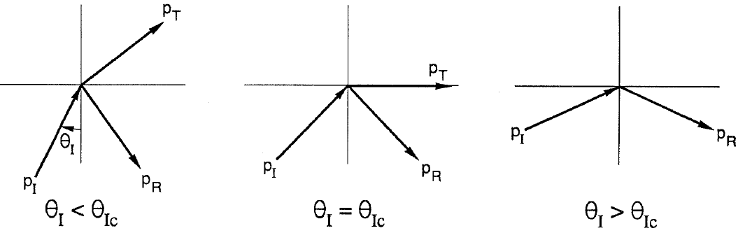
This is called total internal reflection.

Generation of plane waves

At this point, it is natural to ask how these plane waves may be generated. What initial or boundary conditions or forcing terms are needed to generate solutions of the wave equation corresponding to some physical situation? If there are wavemakers in the medium, they can be modelled by body forces $\vec F/\rho_0$ and mass sources $Q$ $$\begin{aligned} \vec u_t & =-\nabla p/\rho_0+\vec F/\rho_0, \\ \rho_t+\rho_0\nabla\cdot\vec u & =Q. \end{aligned}$$ Combining these with $p_t=c^2\rho_t$ yields $$p_{tt}-c^2\nabla^2p=c^2(Q_t-\nabla\cdot\vec F).$$

We can now consider two types of problems: initial value problems and those forced from rest. In both types we solve the homogeneous wave equation while satisfying $\partial p/\partial n=0$ on the solid boundaries and requiring outgoing waves at infinity, i.e. a radiation condition. For the initial value problems, $p$ and $p_t$ are specified at time $t=0$, while for those forced from rest they are set to zero. Of course, there is not really a fundamental distinction because solutions of one type may be linearly superposed to obtain solutions to the other type. The solution procedures may, however, be quite different.

An initial value problem

Let us consider a one-dimensional initial value problem $$p_{tt}-c^2p_{xx}=0\qquad -\infty<x<\infty$$ $$p(x,0)=P_0(x)\ ;\qquad p_t(x,0)=Q_0(x).$$

We will solve this by the method of characteristics. The most general solution is $$p=f(x-ct)+g(x+ct).$$ To satisfy the initial conditions $$\begin{aligned} f(x)+g(x) & =P_0(x), \\ -cf'(x)+cg'(x) & =Q_0(x). \end{aligned}$$ The second integrates to $$f(x)-g(x)=-\frac1c\int_0^x Q_0(x')\,dx'+K$$ whence $$\begin{aligned} 2f(x) & =P_0(x)-\frac1c\int_0^x Q_0(x')\,dx'+K, \\ 2g(x) & =P_0(x)+\frac1c\int_0^x Q_0(x')\,dx'-K. \end{aligned}$$ These give the solution as $$p(x,t)=\frac12\left[P_0(x-ct)+P_0(x+ct) +\frac1c\int_{x-ct}^{x+ct}Q_0(x')\,dx'\right].$$ Note that $p(x,t)$ depends only on the initial conditions over the range $x\pm ct$.

If $Q_0(x)=0$, then the solution is very simple $$p(x,t)=\frac12[P_0(x-ct)+P_0(x+ct)]$$ for which case the solution could have been obtained using the Fourier method, although it is not the method of choice in this problem. Set $$p(x,t)=\int_{-\infty}^{\infty}\bar p(k,t)e^{ikx}\,dk.$$ Then $$\bar p_{tt}+c^2k^2\bar p=0$$ $$\bar p(k,0)=\bar P_0(k)\ ;\qquad \bar p_t(k,0)=0.$$

The solution to this problem is $$\bar p(k,t)=\bar P_0(k)\cos(ckt)$$ from which $$\begin{aligned} p(x,t) & =\int_{-\infty}^{\infty}\bar P_0(k)\cos(ckt)e^{ikx}\,dk \\ & =\frac12\int_{-\infty}^{\infty}\bar P_0(k) \left(e^{ikx+ickt}+e^{ikx-ickt}\right)\,dk \\ & =\frac12[P_0(x-ct)+P_0(x+ct)]. \end{aligned}$$ The integration is trivial in this case but not always.

Forcing from rest

Assume that the forcing has the rather simple form $$Q_t-\nabla\cdot\vec F=\delta(x)q_t(t)$$ where $q(t)=q_t(t)=0$ for $t<0$ and $q_t$ is finite. Now we solve $$p_{tt}-c^2p_{xx}=\delta(x)q_t(t)c^2$$ $$p(x,0)=p_t(x,0)=0\qquad\text{at }t=0.$$ We may put the forcing into the boundary condition by $$\int_{0^-}^{0^+}(p_{tt}-c^2p_{xx})\,dx =-c^2p_x\big|_{0^-}^{0^+}=c^2q_t(t).$$ That is, $p_x(x=0+,t)-p_x(x=0-,t)=-q_t(t)$ so that the forcing at $x=0$ is interpretable as a specified discontinuity there. So we must solve

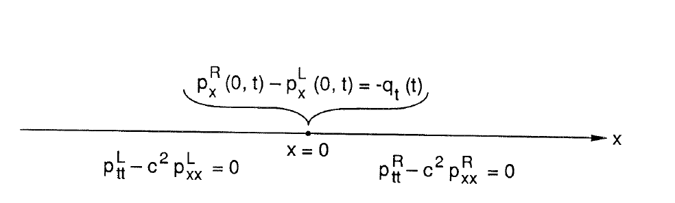
where $p^L$ and $p^R$ are solutions on the left and right of the discontinuity, respectively. Most generally, $p^L$ and $p^R$ are functions of $x\pm ct$. We write them along with the requirement of symmetry $$p^R(x,t)=p^L(-x,t)$$ $$p^R(x,t)=f(x-ct)+g(x+ct)$$ $$p^L(x,t)=f(-x-ct)+g(-x+ct).$$ Imposing the jump condition at $x=0$ yields $$f'(-ct)+g'(ct)+f'(-ct)+g'(ct)=-q_t(t)$$ but this does not specify $f$ and $g$. To specify them, we must impose a radiation condition, i.e., $$p^R(x,t)=f(x-ct)\qquad p^R\text{ is all right going waves}$$ $$p^L(x,t)=f(-x-ct)\qquad p^L\text{ is all left going waves}.$$ Now we have $$2f'(-ct)=-q_t(t)$$ $$2f(-ct)=q(t)c$$ $$f(\tau)=\frac{c}{2}q(-\tau/c).$$

from which $$p^R(x,t)=\frac{c}{2}q(-x/c+t)$$ $$p^L(x,t)=\frac{c}{2}q(x/c+t).$$ Thus, forcing at the origin is modelled as a jump in $p_x$ and we must assume that all of the motion is away from the source in order to get a unique answer.

If the forcing were harmonic with $q(t)=e^{-i\sigma t}/(-i\sigma)$ then $$p_{tt}-c^2p_{xx}=c^2\delta(x)e^{-i\sigma t}$$ and the solution would be $$p^R(x,t)=\frac{-c}{2(i\sigma)}e^{-i\sigma(-x/c+t)}$$ $$p^L(x,t)=\frac{-c}{2(i\sigma)}e^{-i\sigma(x/c+t)}.$$ In other words, plane waves radiating outwards from $x=0$. The radiation condition that we imposed models a little bit of dissipation in the sense that the solution looks dissipationless locally, but nothing is reflected from $|x|\to\infty$ because even small dissipation attenuates any reflected waves over a long distance. We could, in fact, add a friction term to the momentum equations and solve again to obtain a solution which would become the present solution for vanishingly small friction.

Slowly varying medium

We have considered cases in which the speed of sound remains constant in the medium or changes abruptly at an interface. However, the speed of sound within the ocean varies in space because the ocean is not a uniform fluid. In fact the sound speed in the

ocean is sensitive to the temperature, salinity and pressure of the ocean and may be described by the following empirical formula: $$c(s,T,z)=c_0+\alpha_0(T-10)+\beta_0(T-10)^2+\gamma_0(T-18)^2 +\delta_0(s-35)+\epsilon_0(T-18)(s-35)+\zeta_0|z|$$ where the coefficients have the appropriate mks units and have values of $$c_0=1493.0,\quad \alpha_0=3.0,\quad \beta_0=-0.006,\quad \gamma_0=-0.04, \quad \delta_0=1.2,\quad \epsilon_0=-0.01,\quad \zeta_0=0.0164.$$ This says that the speed of sound varies quadratically with temperature, and linearly with salinity and depth. The depth effect is due to changes in the ambient pressure. For typical ocean conditions, the temperature effect dominates in the shallow water, while the pressure effect dominates in the deep water. The sound speed increases with an increase in either temperature or depth, so there is typically a sound speed minimum in the ocean interior.

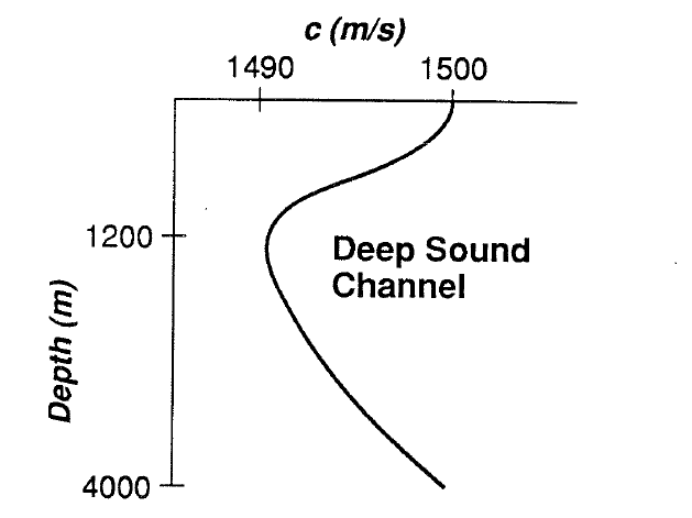
The situation is different in the arctic where there is little effect of warming near the surface. There, the sound speed tends to decrease right up to the surface.

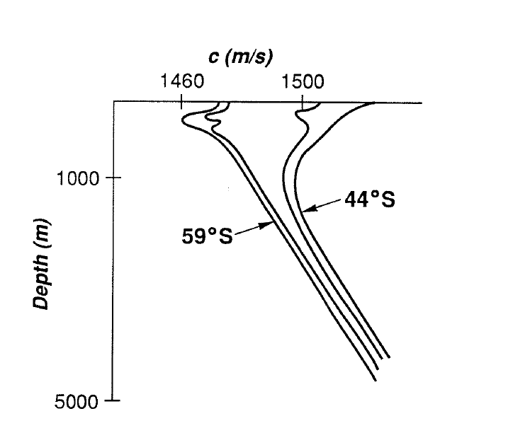
We can examine the effects of these variations in sound speed by applying our knowledge of ray theory. We must assume that the wavelengths of the acoustic waves are much less than the scale over which the sound speed changes. That is, the wavelength must be small compared to the total ocean depth. We will consider only two dimensions, the vertical and one horizontal. Recalling our discussion of ray theory, we write the dispersion relation as $$\sigma=\Omega(k,m;z).$$ Since the medium varies only in $z$, we have $\partial\Omega/\partial x=0$, $\partial\Omega/\partial t=0$ but $\partial\Omega/\partial z\ne0$. Thus, the ray equations become $$\begin{aligned} \frac{dN}{dt} & =0, \\ \frac{dk}{dt} & =0, \\ \frac{dm}{dt} & =-\frac{\partial\Omega}{\partial z}. \end{aligned}$$ These say that the component of the wavenumber in the $x$ direction remains constant in time (which makes sense since the medium varies only in $z$), and that the frequency remains fixed at the initial frequency. We could integrate these following along a ray

with the group velocity, but we will examine the qualitative behavior by considering Snell’s Law which can be derived in the same manner as for the case of scattering at the discontinuity. The frequency can be written in terms of the angle that the wavenumber makes with the vertical to obtain $$\frac{\sin\theta_0}{c_0}=\frac{\sin\theta}{c(z)}$$

or $$\sin\theta=\frac{c(z)}{c_0}\sin\theta_0$$ where $c_0$ and $\theta_0$ are the initial values.

Consider the case in which the sound speed decreases with depth, $c=c_0(1+\alpha z)$ (remember that $z$ is positive upwards). This means that a wave moving upward moves into a region of increasing sound speed, so the angle with the vertical must increase as well. Thus, the wave moves toward a horizontal path. This may also be seen from the ray equations where $-\partial\Omega/\partial z<0$, so that $m$ must decrease with upward motion. Decreasing $m$ leads to a more horizontal propagation path.

Similarly if $c$ increases in the deep ocean, sound waves moving downward will be turned toward the horizontal.

When the ray becomes nearly horizontal, ray theory must be applied very carefully. From the ray definition, we can write $$\frac{dz}{dx}=\frac{c_{gz}}{c_{gx}} =\frac{\partial\Omega/\partial m}{\partial\Omega/\partial k} =\frac{m}{k} =\left(\frac{\sigma^2}{c^2(z)k^2}-1\right)^{1/2}$$

which gives the slope of the ray path. This may be approximated near the critical level $z_c$ by expanding in a Taylor series to obtain $$\frac{dz}{dx}\simeq \left[ (z-z_c)\frac{d}{dz}\left(\frac{\sigma^2}{c^2(z)k^2}\right)_{z=z_c} \right]^{1/2}$$ which integrates to $$z=z_c+\frac14 \left[\frac{d}{dz}\left(\frac{\sigma^2}{c^2(z)k^2}\right)\right]_{z=z_c} (x-x_0)^2.$$ Thus, the ray path is parabolic near the critical level, so an upward propagating ray turns downward.

Similarly, a downward propagating ray which encounters an increasing $c$ at depth will eventually turn upward (provided it does not intersect the bottom). The end result is that the minimum in the sound speed acts as a sound channel where acoustic energy can propagate over hundreds of kilometers without encountering the bottom provided the incidence angle is not too oblique. Numerous examples are reproduced in Apel (1987). This is the basis of acoustic tomography, in which this efficient propagation is used to infer properties of the ocean. Sound waves are generated at a source and received at a listening station. For a fixed vertical profile of the sound speed, the rays may be calculated using ray theory. The received signal is then compared with that expected for a horizontally uniform medium, and differences are used to deduce various physical phenomena which might have occurred along the ray paths. This is generally called an inverse problem because boundary observations are used to determine the interior physics, rather than the reverse.