Internal gravity waves

We have seen that gravity can provide the restoring force which allows waves to propagate along an interface. We saw that if the interface separates two fluids with slightly different densities, then a much slower version of surface waves — called internal waves — is possible. We now turn our attention to a more thorough investigation of internal gravity waves. In particular, we extend the previous ideas to situations in which the vertical density stratification varies continuously within the fluid. And, since internal waves are ubiquitous in the ocean, we will spend some time reviewing their observed properties, as well.

The internal wave equation

Suppose we do the following thought experiment. In a continuously stratified fluid, we raise a parcel of water from its equilibrium position a small amount $\xi$.

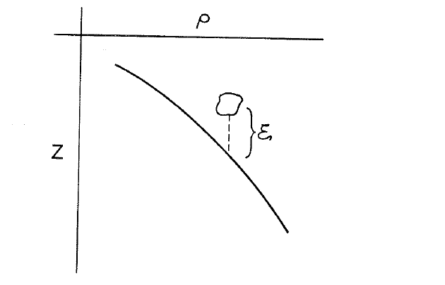
The change in pressure experienced by the parcel is $dp=-\rho_0g\xi$ while the change in density is $d\rho=dp/c^2$. At this point, the buoyancy force acting on the parcel (per unit volume) introduces an acceleration, so that $$g(\rho_{out}-\rho_{in}) =g[(\rho_0+\rho_{0z}\xi)-(\rho_0-\rho_0g\xi/c^2)] =\rho_0\xi_{tt}.$$ Rearranging $$\xi_{tt}+\xi\left(-\frac{g\rho_{0z}}{\rho_0}-\frac{g^2}{c^2}\right)=0$$ which is a simple harmonic oscillator equation with solution $e^{\pm iNt}$ where $$N^2(z)=-\frac{g\rho_{0z}}{\rho_0}-\frac{g^2}{c^2}.$$ Thus the parcel oscillates about its equilibrium position at a natural frequency determined by the local density stratification and the fluid’s compressibility. This frequency is called the buoyancy, Brunt–Väisälä or Väisälä frequency and is often used to characterize the degree of stratification in the ocean.

For applications to the ocean, the effect of compressibility is typically neglected because $g^2/c^2$ is usually small compared to $g\rho_{0z}/\rho$, so we will neglect it here. In the atmosphere, compressibility is often important, so the full definition of $N^2$ must be used. A brief discussion of this case is presented by Gill (1982, pp. 169–175).

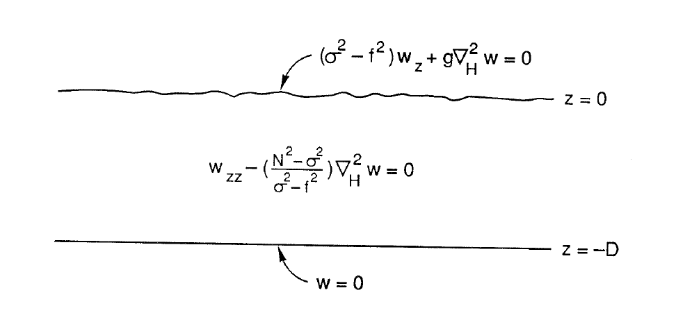
The momentum, mass and continuity equations for a rotating, incompressible fluid are $$\frac{D\vec u^{\,*}}{Dt}+f\hat k\times\vec u^{\,*} =-\frac{\nabla p^*}{\rho^*}-g\hat k$$ $$\frac{\partial\rho^*}{\partial t}+\nabla\cdot\rho^*\vec u^{\,*}=0$$ $$\frac{D\rho^*}{Dt}=0\ \Rightarrow\ \nabla\cdot\vec u^{\,*}=0.$$ One solution to these equations is a motionless, hydrostatic balance, i.e. $\vec u_0=0$; $0=-p_{0z}-g\rho_0(z)$. Each dynamic variable may then be separated into a hydrostatic part and a small departure from it $$\vec u^{\,*}=\vec u_0+\vec u\ ;\qquad p^*=p_0+p\ ;\qquad \rho^*=\rho_0+\rho.$$ After substituting these into the full equations, assuming that the departures are very small perturbations and neglecting the nonlinear terms, we obtain $$\frac{\partial\vec u}{\partial t}+f\hat k\times\vec u =-\frac{\nabla p}{\rho_0}-\frac{g\rho\hat k}{\rho_0}$$ $$\rho_t+w\rho_{0z}=0$$ $$\nabla\cdot\vec u=0.$$ Next we specialize to periodic motion $e^{-i\sigma t}$ and write out components $$\begin{aligned} -i\sigma u-fv & =-p_x/\rho_0, \\ -i\sigma v+fu & =-p_y/\rho_0, \\ -i\sigma w & =-p_z/\rho_0-g\rho/\rho_0, \\ u_x+v_y+w_z & =0, \\ -i\sigma\rho+w\rho_{0z} & =0. \end{aligned}$$ Eliminate $\rho$ between the vertical momentum equation and the density equation $$\rho_0(N^2-\sigma^2)w=i\sigma p_z.$$

The horizontal momentum equations may be rewritten $$u=\frac{1}{\rho_0}\frac{-i\sigma p_x+fp_y}{\sigma^2-f^2}$$ $$v=\frac{1}{\rho_0}\frac{-i\sigma p_y-fp_x}{\sigma^2-f^2}$$ from which continuity becomes $$-i\sigma\nabla_H^2p+(\sigma^2-f^2)\rho_0w_z=0$$ where $\nabla_H^2=\partial^2/\partial x^2+\partial^2/\partial y^2$. Now eliminate the pressure to obtain $$\rho_0(N^2-\sigma^2)\nabla_H^2w-(\sigma^2-f^2)(\rho_0w_z)_z=0$$ or $$\frac{1}{\rho_0}(\rho_0w_z)_z -\left(\frac{N^2-\sigma^2}{\sigma^2-f^2}\right)\nabla_H^2w=0.$$ Now if we had let $\rho_0$ be constant in the momentum equations [so that it is differentiated only in $N^2(z)$], then we would have obtained $$w_{zz}-\frac{N^2-\sigma^2}{\sigma^2-f^2}\nabla_H^2w=0.$$ This last simplification is called the Boussinesq approximation and it means that $\rho_{0z}/\rho_0\ll w_z/w$, i.e. $\rho_0(z)$ changes over a large vertical scale. It is quite adequate in the ocean.

At the free surface (very close to $z=0$), we have $Dp^*/Dt=0$. Let $p^*=p_0+p$, linearize and apply the result at $z=0$: $$-i\sigma p+w p_{0z}=0\qquad\text{at}\qquad z=0$$ or $$-i\sigma p-wg\rho_0=0\qquad\text{at}\qquad z=0.$$ Now use the previous equations to eliminate $p$ $$(\sigma^2-f^2)w_z+g\nabla_H^2w=0\qquad\text{at}\qquad z=0.$$

At a flat bottom $$w=0\qquad\text{at}\qquad z=-D.$$ So we have to solve

Unbounded, rotating, stratified fluid

We suppose for the moment that $N^2(z)=\text{constant}$. We also assume that the coordinates rotate around the $z$ axis at $\Omega$ so that $f=2\Omega=\text{constant}$ which is the $f$-plane approximation. The field equation is $$w_{zz}-\left(\frac{N^2-\sigma^2}{\sigma^2-f^2}\right)(w_{xx}+w_{yy})=0.$$

Since $N,f$ are constants, exact solutions are $$w=e^{-i\sigma t+ikx+i{ℓ} y+imz}$$ from which $$m^2=\left(\frac{N^2-\sigma^2}{\sigma^2-f^2}\right)(k^2+{ℓ}^2)$$

is the dispersion relation. In $k,{ℓ},m$ space, the dispersion relation is a cone if $f^2<\sigma^2<N^2$ or $f^2>\sigma^2>N^2$.

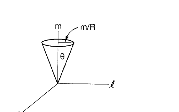
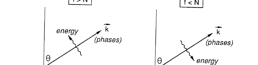
All possible wave vectors for waves of frequency $\sigma$ lie on this cone. They may have any length. Fixing $\sigma$ fixes their direction. If we define $\theta$ as in the sketch, then with $K=(k^2+{ℓ}^2+m^2)^{1/2}$, we can write $$m=K\cos\theta\ ;\qquad (k^2+{ℓ}^2)^{1/2}=K\sin\theta$$ and the dispersion relation may be rewritten as $$\sigma^2=N^2\sin^2\theta+f^2\cos^2\theta$$ or $$\sigma^2K^2=N^2(k^2+{ℓ}^2)+f^2m^2.$$ These waves are of the form $(\vec u,p,\rho)=(\vec u_0,p_0,\rho_0)e^{-i\sigma t+i\vec k\cdot\vec x}$. By continuity, $\nabla\cdot\vec u$ leads to $\vec k\cdot\vec u_0=0$ which means that the fluid motion occurs in planes normal to the wave vector. That is, the waves are transverse. Also, $\nabla p\sim\vec k p_0$ which is perpendicular to $\vec u$, so the pressure gradient forces are normal to fluid flow and acceleration.

If $f=0$, then the momentum equation in any direction normal to $\vec k$

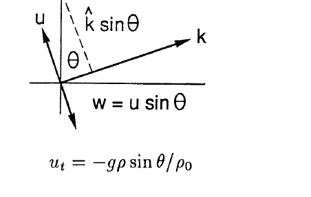
becomes $$u_t=-gp\sin\theta/\rho_0$$

while $$\rho_t+u\sin\theta\,\rho_{0z}=0$$ because the pressure gradient forces are along $\vec k$. This says that only the density gradient along $\vec u$ matters, from which $$u_{tt}+N^2\sin^2\theta\,u=0\ ;\qquad \sigma^2=N^2\sin^2\theta$$ and motion is along a straight line perpendicular to $\vec k$.

If $N=0$, then the momentum equation in any direction normal to $\vec k$

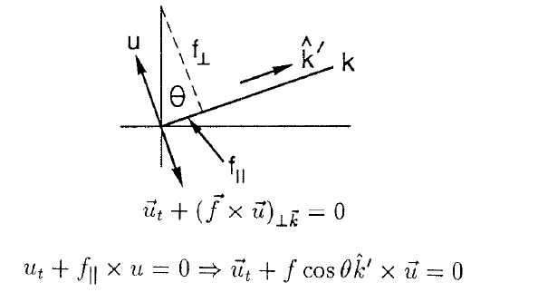
becomes $$\vec u_t+f\cos\theta\,\hat k'\times\vec u=0.$$ Thus the motion occurs in inertial circles at $\sigma^2=f^2\cos^2\theta$.

We can examine the group velocity by defining $$W(k,{ℓ},m,\sigma) =m^2-\frac{N^2-\sigma^2}{\sigma^2-f^2}(k^2+{ℓ}^2)=0.$$ Now $$dW\big|_{{ℓ},m} =\frac{\partial W}{\partial k}\,dk +\frac{\partial W}{\partial\sigma}\,d\sigma=0$$

so $$\left.\frac{\partial\sigma}{\partial k}\right|_{{ℓ},m} =-\frac{\left.\partial W/\partial k\right|_{{ℓ},m}} {\left.\partial W/\partial\sigma\right|_{{ℓ},m}} \qquad\text{etc.}$$ From this $$\begin{aligned} c_{gx} & =\frac{\partial\sigma}{\partial k} =\frac{k}{\sigma}\frac{N^2-\sigma^2}{K^2}, \\ c_{gy} & =\frac{\partial\sigma}{\partial{ℓ}} =\frac{{ℓ}}{\sigma}\frac{N^2-\sigma^2}{K^2}, \\ c_{gz} & =\frac{\partial\sigma}{\partial m} =-\frac{m}{\sigma}\frac{\sigma^2-f^2}{K^2}. \end{aligned}$$ First notice that $$\begin{aligned} \vec k\cdot\vec c_g & =\left(\frac{k^2}{\sigma}+\frac{{ℓ}^2}{\sigma}\right) \left(\frac{N^2-\sigma^2}{K^2}\right) -\frac{m^2}{\sigma}\left(\frac{\sigma^2-f^2}{K^2}\right) \\ & =\frac{-\sigma^2(k^2+{ℓ}^2+m^2)+N^2(k^2+{ℓ}^2)+f^2m^2}{K^2\sigma} \\ & =0. \end{aligned}$$ This means that the group velocity is perpendicular to the phase velocity! Next observe that $$\vec c_g=\frac{1}{\sigma K^2} [\hat i k(N^2-\sigma^2)+\hat j{ℓ}(N^2-\sigma^2) +\hat k m(f^2-\sigma^2+N^2-N^2)]$$ That is $$\vec c_g=\frac{1}{\sigma K^2} [\vec k(N^2-\sigma^2)-\hat k m(N^2-f^2)].$$ This allows us to visualize the direction of $\vec c_g$.

Finally, using the dispersion relation, $$\begin{aligned} |\vec c_g| & =\left(c_{gx}^2+c_{gy}^2+c_{gz}^2\right)^{1/2} \\ & =\frac{[k^2(N^2-\sigma^2)^2+{ℓ}^2(N^2-\sigma^2)^2 +m^2(\sigma^2-f^2)^2]^{1/2}}{\sigma K^2} \\ & =\frac{[(N^2-\sigma^2)^2\sin^2\theta +(\sigma^2-f^2)^2\cos^2\theta]^{1/2}}{\sigma K} \\ & =\frac{[(N^2-f^2)^2\sin^4\theta\cos^2\theta +(N^2-f^2)^2\cos^4\theta\sin^2\theta]^{1/2}}{\sigma K} \\ & =\frac{|N^2-f^2|\sin\theta\cos\theta}{\sigma K}. \end{aligned}$$ An alternative is to define $\phi$ as the angle of energy propagation such that $$\sigma^2=N^2\cos^2\phi+f^2\sin^2\phi$$ $$|\vec c_g|=|N^2-f^2|\sin\phi\cos\phi/(\sigma K).$$

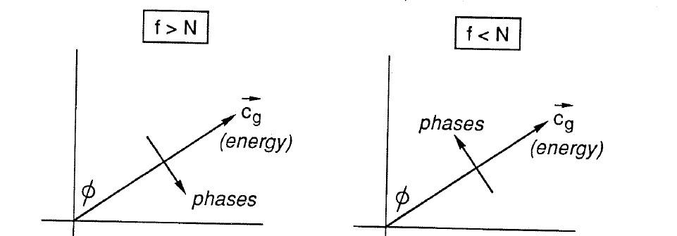
There is really nothing mysterious about $\vec c_g,\vec c_{ph}$. For deep water waves we had

$c_g=\frac12c_{ph}$ which states that, in a group, individual crests arise at the trailing end, propagate through the group faster than the group goes, and die out at the leading edge. For these internal gravity waves, individual crests arise at one side of the group and move through it at right angles to the group motion, finally dying out at the other side. An example is depicted by Gill (1982, pp. 135–6).

Imagine a harmonic source $e^{-i\sigma t}$ at the origin of space coordinates and let’s discuss the wave field for various choices of $\sigma,N,f$. In the general case, energy is localized to the cone whose apex angle is $\phi$ defined by $\sigma^2=N^2\cos^2\phi+f^2\sin^2\phi$.

(i) Rotation only: $N=0$, $f\ne0$. We have $$\sigma=f\sin\phi\ ;\qquad |\vec c_g|=f\cos\phi/K.$$

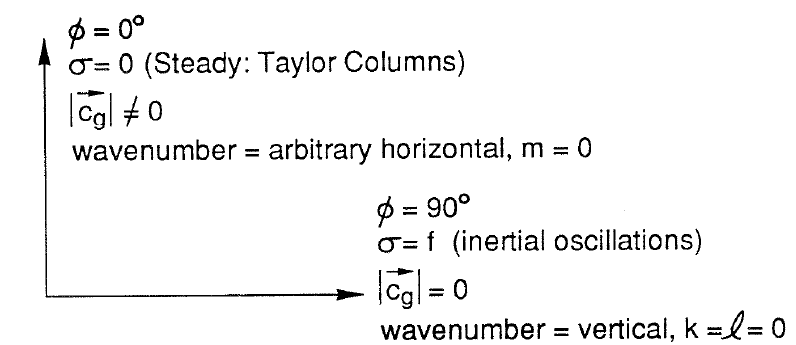
This says that for vertical energy propagation, $\phi=0^\circ$, the flow is steady ($\sigma=0$) but the group velocity is nonzero. The wavenumbers are arbitrary but horizontal, i.e. $m=0$. The flow is basically that of Taylor columns which are steady, geostrophic flows with no vertical variability ($\partial/\partial z=0$). If the direction of energy propagation is horizontal, $\phi=90^\circ$, then the frequency must be the inertial frequency ($\sigma=f$) and the group velocity is zero. The wavenumber is purely vertical, i.e. $k={ℓ}=0$. This corresponds to solutions of the horizontal momentum equations in which $p$ is a function of $z$ only. The pressure gradient terms disappear leaving $$u_t-fv=0$$

$$v_t+fu=0$$ which has the solution $\sigma=f$, $u=iv$. Thus, we see that in a rotating homogeneous fluid, low frequency energy flows vertically in the form of Taylor columns, while inertial oscillations at different depths are entirely independent.

(ii) Stratification only: $f=0$, $N\ne0$. We have $$\sigma=N\cos\phi\ ;\qquad |\vec c_g|=N\sin\phi/K.$$

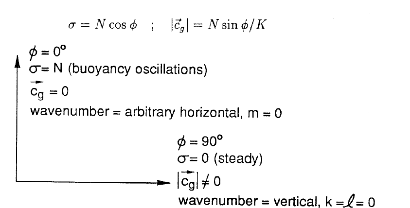
This says that for vertical energy propagation, $\phi=0^\circ$, the flow oscillates at the buoyancy frequency ($\sigma=N$) and the group velocity is zero. The wavenumber is arbitrary and horizontal, i.e. $m=0$. These are called buoyancy oscillations. The flow has Taylor column-like structure, columnar in the vertical, but it is like inertial oscillations in that energy does not propagate. For horizontal energy propagation, $\phi=90^\circ$, the flow is steady ($\sigma=0$) and the group velocity is nonzero. The wavenumber is vertical. In this case, the momentum equations reduce to $0=-\nabla p/\rho_0-\hat k g\rho/\rho_0$ from which $\rho$ must be zero since it does not vary in time and can be absorbed into $\rho_0$. This leads to $w=0$ from the density equation, leaving $u_x+v_y=0$ from continuity. So, each layer in the stratified flow moves independently of all others. Flow in each layer is nondivergent and buoyancy has no effect. In two dimensions, if $v_y=0$ ($v=0$, say), then $u_x=0$, i.e. $u=u(z)$. Thus, low frequency energy flows horizontally and, in two dimensions, is analogous to the Taylor column flows.

Notice quite generally that effects due to $f$ and effects due to constant $N$ are very similar in their mathematical expression.

(iii) Both rotation and constant stratification: $$\sigma^2=N^2\cos^2\phi+f^2\sin^2\phi$$ $$|\vec c_g|=|N^2-f^2|\sin\phi\cos\phi/(\sigma K).$$

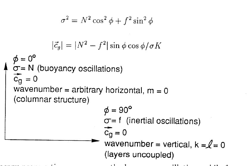
For vertical energy propagation, we recover the buoyancy oscillations while for horizontal energy propagation, we recover the inertial oscillations. Now there are no zero frequency wave flows that propagate energy. At frequency $\sigma$, energy is confined to the cone whose sides lie at $\phi$ to the vertical.

What happens if the source frequency is outside the range of $f$ to $N$? In that case the field equation can be written $$w_{zz}+\frac{\sigma^2-N^2}{\sigma^2-f^2}(w_{xx}+w_{yy})=0$$ and we see that the very nature of the equation has changed from a hyperbolic (or wave-type) equation to an elliptic (or potential flow type) equation because the sign of the coefficient has changed. Our free-wave dispersion relation now becomes $$m^2=-\frac{\sigma^2-N^2}{\sigma^2-f^2}(k^2+{ℓ}^2).$$

and we see that at least one of the wavenumbers must be complex. This, in turn, means that the solution is no longer free to propagate, but instead must decay exponentially in some direction. For example, for waves propagating in the horizontal ($k,{ℓ}$ are real), the oscillations must grow or decay monotonically in the vertical.

Waveguide modes

We turn our attention to the full problem introduced at the beginning of the chapter. Instead of an unbounded fluid, there are now surface and bottom boundaries to contend with.

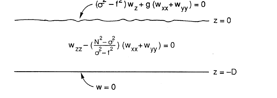
Initially we restrict ourselves to $N^2=\text{constant}$. The signs of $$S^2\equiv\sigma^2-f^2\ ;\qquad R^2\equiv\frac{N^2-\sigma^2}{\sigma^2-f^2}$$ are crucial and we have several cases to consider.

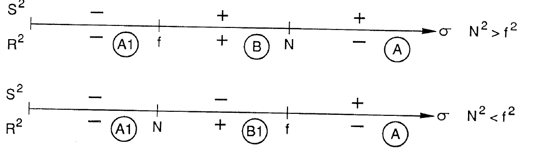
Evidently the cases $\sigma^2>N^2,f^2$ and $\sigma^2<N^2,f^2$ are identical for either $N^2>f^2$ or $N^2<f^2$, but the case where $\sigma^2$ is intermediate between $N^2$ and $f^2$ depends strongly on whether $N^2>f^2$ or $N^2<f^2$. We will look at cases A and B separately.

Case A: Define $R_1^2=(\sigma^2-N^2)/(\sigma^2-f^2)$ and consider $R_1^2>0$. We let $$w=e^{-i\sigma t+ikx}\omega(z)$$ and $\omega$ satisfies $$(\sigma^2-f^2)\omega_z-gk^2\omega=0\qquad z=0$$ $$\omega_{zz}-k^2R_1^2\omega=0$$ $$\omega=0\qquad z=-D.$$ Solutions are $$w=e^{-i\sigma t+ikx}\sinh[kR_1(z+D)]$$ and they satisfy the top ($z=0$) boundary condition only if $$\frac{R_1(\sigma^2-f^2)}{gk}=\tanh(kR_1D).$$

This last relation is effectively the dispersion relation; its solution is $\sigma=\sigma(k)$ or, as we have done the problem, $k=k(\sigma)$. To see what solutions exist, plot the left-hand side and the right-hand side versus $k$.

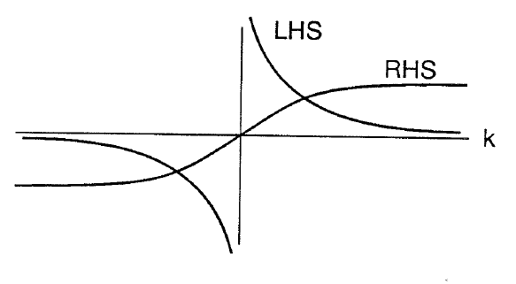
This is case A with $S^2=\sigma^2-f^2>0$. There are two oppositely travelling waves which we can identify with the usual surface waves existing in the absence of stratification and rotation. $$N^2=f^2=0\ ;\qquad R_1^2=1\ ;\qquad \sigma^2-f^2=\sigma^2>0.$$ Notice that in case A1 ($\sigma^2<f^2,N^2$), no waves exist. The plot of the left-hand side and the right-hand side versus $k$ looks like

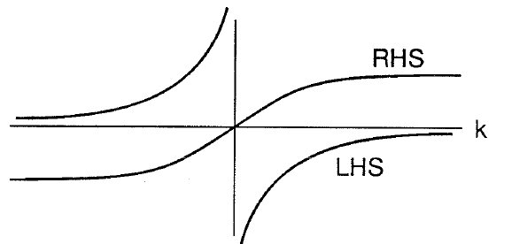
and there are no solutions to the proposed dispersion relation. What has happened is that our assumption of free wave propagation in the $x$ direction (real $k$) has proved impossible to satisfy.

Case B: Now $R^2=(N^2-\sigma^2)/(\sigma^2-f^2)>0$. We let $$w=e^{-i\sigma t+ikx}\omega(z)$$ and $\omega$ satisfies $$(\sigma^2-f^2)\omega_z-gk^2\omega=0\qquad z=0$$ $$\omega_{zz}+k^2R^2\omega=0.$$

$$\omega=0\qquad z=-D.$$ Solutions this time are $$w=e^{-i\sigma t+ikx}\sin[kR(z+D)]$$ with $$\frac{R(\sigma^2-f^2)}{gk}=\tan(kRD).$$ Again we look at the dispersion relation

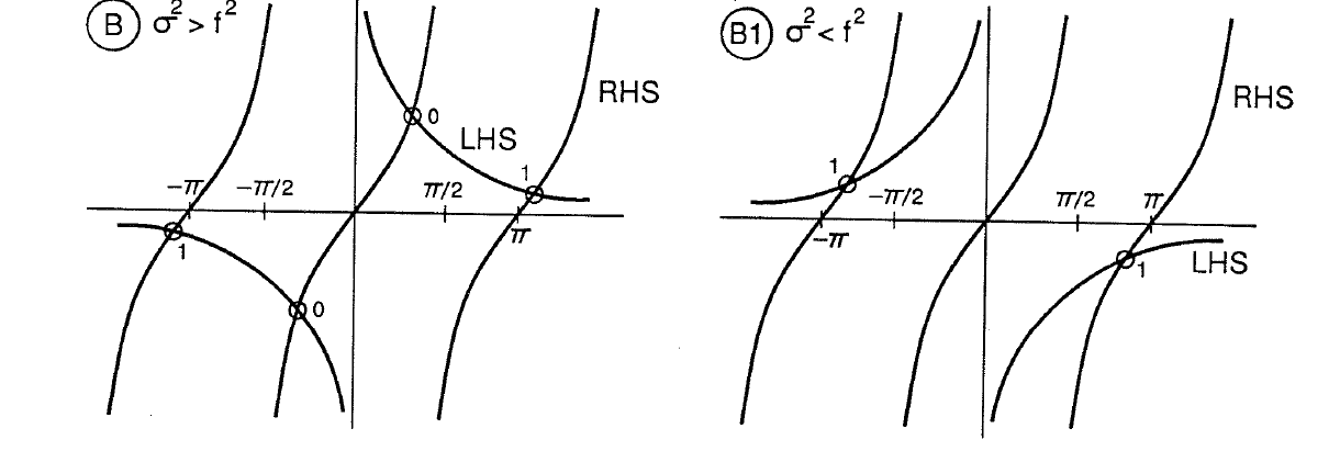
In both cases there is now an infinite set of oppositely travelling modes $n=1,2,\ldots$. The case $\sigma^2>f^2$ has an additional pair of small-$k$ modes not present in the case $\sigma^2<f^2$.

For large $k$, the $n=1,2,\ldots$ modes have the approximate dispersion relation $$k_nRD=\pm n\pi,$$ or $$k_nD\left(\frac{N^2-\sigma^2}{\sigma^2-f^2}\right)^{1/2}=\pm n\pi.$$ This does not hold for the small $k$ ($n=0$) modes. For them, if $kRD\ll1$, then we obtain $$\frac{\sigma^2-f^2}{gD}=k_0^2.$$ These we recognize as the old surface modes in shallow water now modified by rotation. Note that they do not exist when $\sigma^2<f^2$.

Notice that if we require $w=\omega=0$ at $z=0$, i.e. a rigid lid, then the dispersion relation is $\sin(kRD)=0$, so that $k_nRD=\pm n\pi$ becomes exact. But we no longer have the surface modes $k_0$.

Let’s look at the dispersion relations more closely. For the surface modes $$\sigma^2\simeq k^2gD+f^2.$$ For the internal modes $$(\sigma^2-f^2)(n\pi/kD)^2\simeq(N^2-\sigma^2)$$ $$\sigma^2[1+(n\pi/kD)^2]\simeq N^2+f^2(n\pi/kD)^2.$$

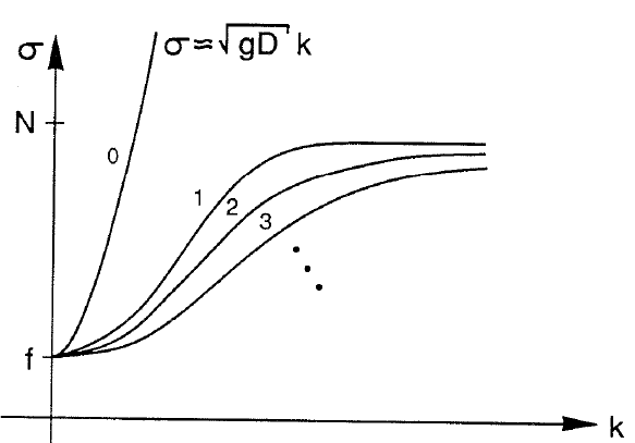
Note that all waves have $\sigma>f$ and that all internal modes have $\sigma<N$. These two limits are also points of vanishing $\vec c_g$ which is easily seen since $\partial\sigma/\partial k\to0$ there.

It is useful to examine the kinematics of the internal modes. We have $$w=w_0e^{-i\sigma t+ikx}\sin[kR(z+D)].$$ From continuity ($u_x+w_z=0$) $$u=iRw_0e^{-i\sigma t+ikx}\cos[kR(z+D)].$$

Consider the lowest mode $n=1$. Then from the dispersion relation $k_1\simeq\pi/RD$ and $$w=w_0\cos(k_1x-\sigma t)\sin[\pi(z+D)/D]\ ;\qquad u=-Rw_0\sin(k_1x-\sigma t)\cos[\pi(z+D)/D]$$ after taking the real part. The vertical structure looks like

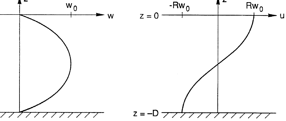
Thus, we see that the particle motions under the crest and trough of a travelling wave consists of a series of convergences and divergences giving a system of vertical cells.

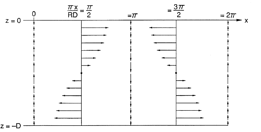
One common consequence of this pattern is the formation of surface slicks or bands of smooth, unrippled surface water, the bands being aligned parallel to the internal wave crests. The scenario is as follows. A very thin organic film (one or two molecules thick)

typically covers the water surface. The periodic convergences and divergences of the horizontal surface current due to the internal waves produce periodic contractions and expansions of the surface film. This leads to an increase in the amount of film over the convergences. The effect of the film in general is to reduce the surface tension, thereby decreasing the tendency for short surface and capillary waves to form as the wind blows over the water. Thus, the region over the convergences tends to have less ripples almost to the point of elimination. These are the surface slicks. Such surface slicks have often been used to infer the presence of internal waves, especially internal solitary waves.

Evanescent modes

We can reexamine the cases considered above but assuming that the wave decays in the $x$ direction. For case A, we have $$w=e^{-i\sigma t+kx}\omega(z)$$ $$(\sigma^2-f^2)\omega_z+gk^2\omega=0\qquad\text{at }z=0$$ $$\omega_{zz}+k^2R_1^2\omega=0$$ $$\omega=0\qquad\text{at }z=-D.$$ Solutions are $$w=e^{-i\sigma t+kx}\sin[kR_1(z+D)]$$ $$\frac{R_1(\sigma^2-f^2)}{gk}=-\tan kR_1D.$$

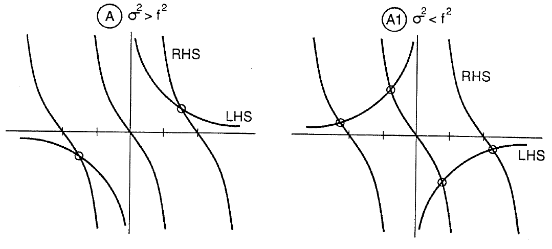
There is an infinite set of evanescent modes although case A1 has two more than case A. Putting on the rigid lid reduces A1 to A, i.e. $\sin(kR_1D)=0$.

For case B, we have $$w=e^{-i\sigma t+kx}\omega(z)$$ $$(\sigma^2-f^2)\omega_z+gk^2\omega=0\qquad\text{at }z=0$$ $$\omega_{zz}-k^2R^2\omega=0$$ $$\omega=0\qquad\text{at }z=-D.$$ Solutions are $$w=e^{-i\sigma t+kx}\sinh[kR(z+D)]$$ $$\frac{R(\sigma^2-f^2)}{gk}=-\tanh kRD.$$

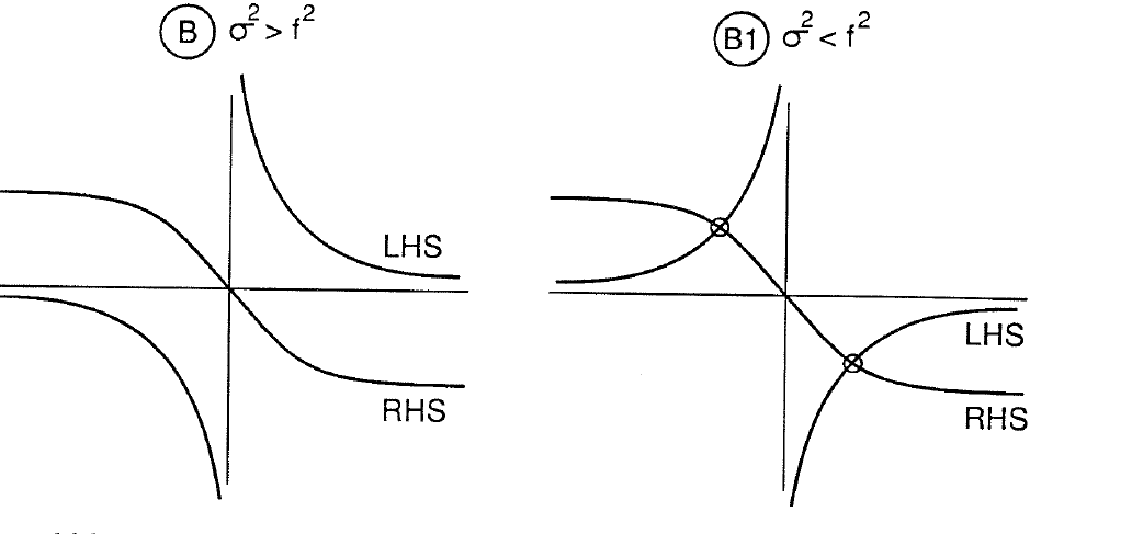
We could have arrived at these same evanescent modes by setting $k=-ik'$ in the previous section.

A summary of internal wave properties for all of the various ranges of parameters can be found in Gill (1982, p. 261).

Generation at a horizontal boundary

We have discussed the properties of freely propagating internal gravity waves, but we have not discussed how these waves might be generated in the ocean or the atmosphere. One way that internal waves are generated is by a mean horizontal flow passing over some topographic feature which forces the flow to move up and down slightly. The following example illustrates this mechanism.

For simplicity, we neglect the effects of rotation and consider two-dimensional flow over a sinusoidally varying horizontal boundary at $z=0$. The amplitude of the variations is assumed small so that the dynamics can be linearized. Of course, an arbitrarily shaped boundary could be used by first Fourier decomposing it, then solving for the flow over each individual component, and then summing the results.

The mean flow has magnitude $U$ in the $x$ direction.

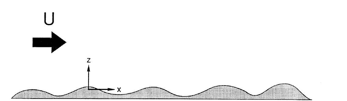
The topography has the form $h=h_0\sin(kx)$ with amplitude $h_0$. Moving along with the mean flow, the topography has the form $$h=h_0\sin[k(x+Ut)]$$ from which we see that the frequency of the resulting motions will be $$\sigma=-Uk.$$ The topography introduces a vertical velocity because the particles near the boundary must follow, to some extent, the undulations of the boundary. So, $$w=U\frac{\partial h}{\partial x}=w_0e^{-i\sigma t+ikx} \qquad\text{on}\qquad z=0.$$ This says that $w_0=Ukh_0$. The field equation for the region above the boundary is $$w_{zz}-\frac{N^2-\sigma^2}{\sigma^2}w_{xx}=0.$$ A solution is $$w=w_0e^{-i\sigma t+ikx+imz}$$ where $$m^2=k^2(N^2-\sigma^2)/\sigma^2=(N/U)^2-k^2$$

after substituting for $\sigma^2$. This solution satisfies the boundary condition at $z=0$ and represents waves with phases propagating downward (because $\sigma<0$) which corresponds to energy propagating upward to $z\to\infty$. Thus, the radiation condition at $z\to\infty$ is satisfied, i.e. no energy enters the system from external sources. We now examine two cases.

Suppose $\sigma^2>N^2$ which means $k>N/U$. This corresponds to short wavelengths or undulations on the boundary. In this case $m^2<0$ so that $m$ must be imaginary. The solution becomes $$w=w_0e^{-i\sigma t+ikx-mz}\ ;\qquad m^2=k^2-(N/U)^2$$ where the sign of $m$ is chosen to ensure that the solution remains finite. Recall that $$\rho_0w_{zt}=p_{xx}$$ from the momentum and continuity equations. This produces $$\rho_0i\sigma mw=-k^2p$$ from which $$p=\frac{-\rho_0i\sigma m}{k^2}w =\frac{-\rho_0i\sigma m}{k^2}w_0e^{-i\sigma t+ikx-mz}.$$ We see that $w$ and $p$ are out of phase by $\pi/2$. Therefore, the vertical energy flux, $\overline{wp}=0$, is identically equal to zero, i.e. there is no vertical energy flux. This makes sense because the solution decays exponentially in the vertical, so the waves cannot transport any energy away from the boundary. Instead, the oscillations are trapped at the boundary. If the wavelength is very small ($kU\gg N$), then stratification has little effect and the flow is essentially irrotational.

Suppose $\sigma^2<N^2$ which means $k<N/U$. This corresponds to longer wavelengths or undulations on the boundary. Now $m^2>0$, so $m$ is real and $m^2=(N/U)^2-k^2$. The solution is $$w=w_0e^{-i\sigma t+ikx+imz}.$$

The form of this solution says that energy is continually being transported toward $z\to\infty$. We have $\rho_0\sigma mw=-k^2p$, so $$p=\frac{-\rho_0\sigma m}{k^2}w =\frac{-\rho_0\sigma m}{k^2}w_0e^{-i\sigma t+ikx+imz}.$$ Now $w$ and $p$ are in phase, so $\overline{wp}\ne0$ and there is a net upward flux of energy. This produces a drag on the mean flow because the energy must come from the mean flow. The drag per unit surface area is the rate at which horizontal momentum is transferred vertically $$\tau=-\rho_0\overline{uw} =\frac{\overline{wp}}{U} =\frac{-\rho_0\sigma m w_0^2}{2k^2}\frac1U =\frac12\rho_0kh_0^2U^2 \left(\frac{N^2}{U^2}-k^2\right)^{1/2}.$$ The cutoff wavenumber which separates the two cases, $k_c=N/U$, corresponds to the wavelength $2\pi/k_c$ which is the horizontal distance traveled by a particle in one buoyancy period. This says that if the particle encounters multiple crests in the topography during one buoyancy period, then the fluid will be forced to oscillate at such a high frequency (greater than $N$) that no free waves can exist and no net drag will be produced. If the particle stays within a single undulation, then the flow adjustments will be slow enough so that free waves will be radiated away producing a drag on the mean flow.

Reflection from a solid boundary

Here we consider the reflection of an internal gravity wave from a solid boundary which is at some angle to the horizontal. To start, consider the two-dimensional solution $e^{-i\sigma t+ikx+imz}$ which satisfies $$w_{zz}-R^2w_{xx}=0$$

where $R^2=(N^2-\sigma^2)/(\sigma^2-f^2)$ and $m=\pm Rk$. Lines of constant phase are those for which $$-\sigma t+kx\pm Rkz=\text{constant}.$$ That is $$x\pm Rz=(\sigma/k)t+\text{constant}.$$

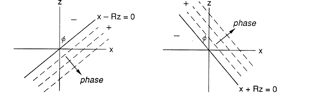
Phases propagate at right angles to $x\pm Rz=\text{constant}$. We see that energy flows along $x\pm Rz=\text{constant}$ because $$z_x=\pm R^{-1} =\pm\left(\frac{\sigma^2-f^2}{N^2-\sigma^2}\right)^{1/2} =\pm\left(\frac{(N^2-f^2)\cos^2\phi} {(N^2-f^2)\sin^2\phi}\right)^{1/2} =\pm\cot\phi.$$ These lines are the characteristics of the hyperbolic $w$ equation, i.e. $$w=F(x+Rz)+G(x-Rz)$$ is the solution.

Now consider reflection from a solid plane wall passing through the origin; $z=ax$. Remember that, for energy incident along $x+Rz=0$, the incident wavenumber is along the normal to that line.

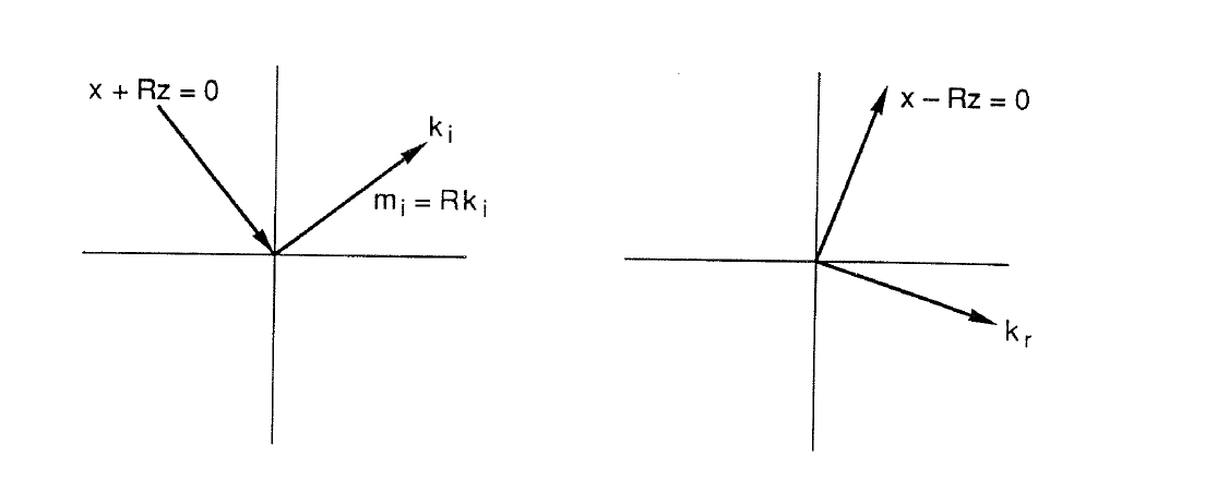
Energy exits along $x-Rz=0$, so the reflected wavenumber is normal to that line. The frequency of the wave is determined solely by the angle to the vertical, and it cannot change upon reflection. Thus the incident and reflected waves must make equal angles with the rotation vector or the vertical (gravity) rather than with the normal to the surface. Therefore, the reflection is not specular.

Consider the details of the situation. The incident wave is $\vec k_i$ and the reflected wave is $\vec k_r$.

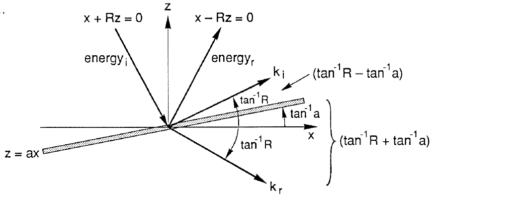
The projection of incident and reflected wavenumbers along $z=ax$ must be equal. $$|\vec k_i|\cos(\tan^{-1}R-\tan^{-1}a) =|\vec k_r|\cos(\tan^{-1}R+\tan^{-1}a).$$ We can evaluate these by geometry and the law of cosines [$\cos\theta=(a^2+b^2-c^2)/2ab$].

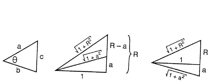
After some algebra, the result is $$|\vec k_r|=|\vec k_i|\left(\frac{1+aR}{1-aR}\right).$$

$$m_r=\pm m_i\left(\frac{1+aR}{1-aR}\right) \left(\frac{R+a}{R-a}\right).$$ where the signs have been taken from the sketch. This gives the new wavenumbers in terms of the old ones. Because waves of a given frequency $\sigma$ can only go in the two directions $\pm\tan^{-1}R$, reflection occurs not in the normal to the reflecting surface, but rather in the direction of the stability gradient, i.e. in the $z$ direction, or in the rotation vector. We have

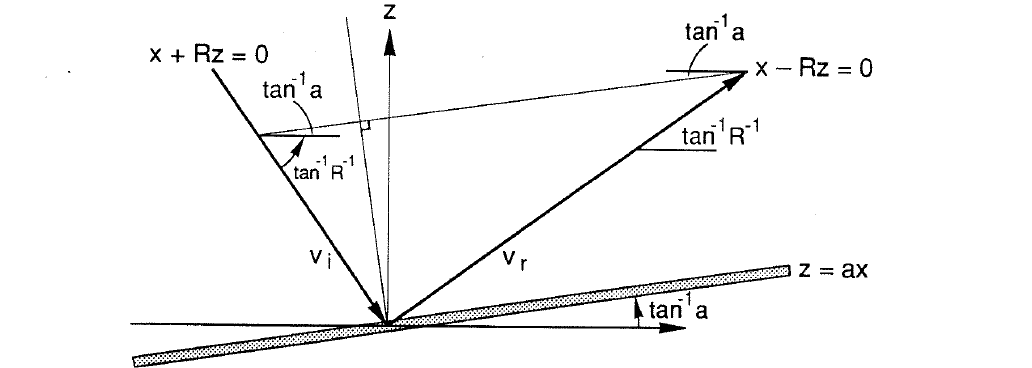
The normal component of velocity must vanish at the wall, so $$|\vec v_i|\sin(\tan^{-1}R^{-1}+\tan^{-1}a) =|\vec v_r|\sin(\tan^{-1}R^{-1}-\tan^{-1}a).$$ Again we can use geometry to obtain $$|\vec v_r|=|\vec v_i|\left(\frac{1+aR}{1-aR}\right).$$

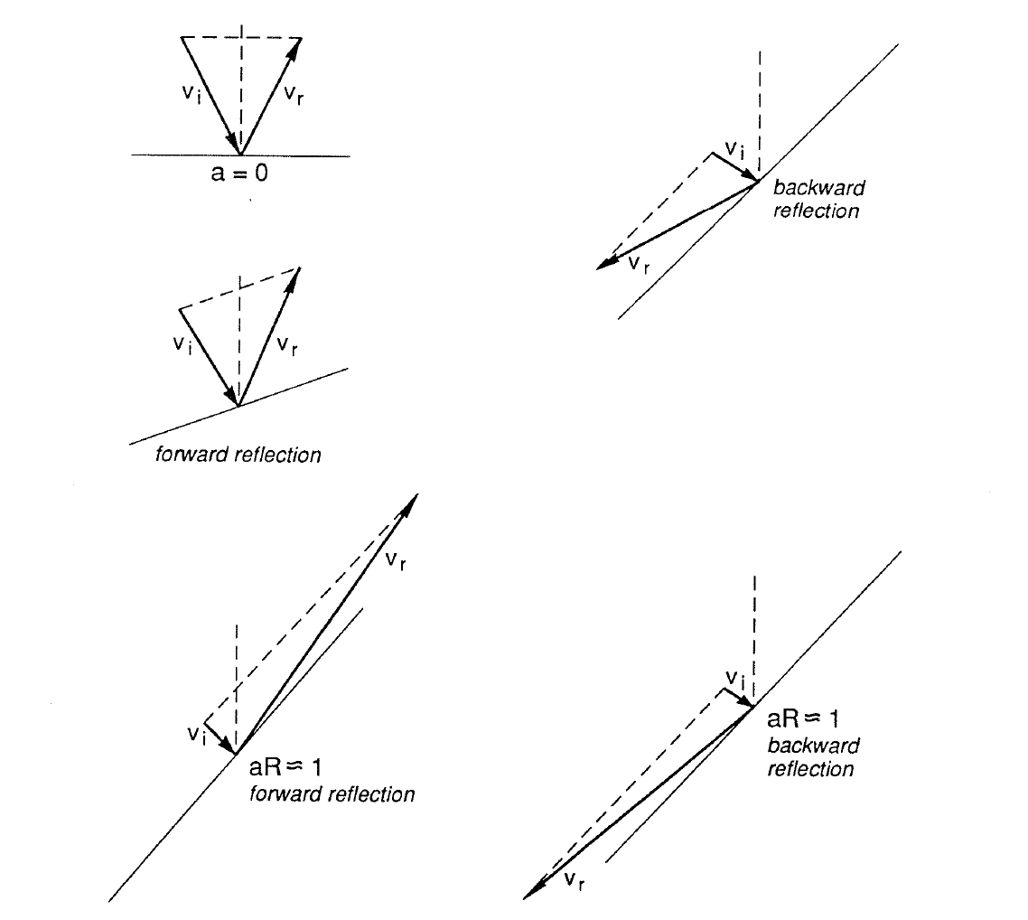
Notice that if $aR=1$, the reflected velocity is very large. What does this mean? It means that the bottom coincides with the outgoing characteristic; $z=ax$ is the bottom and the outgoing characteristic has the same slope. So, as $aR\to1$, $|\vec v_r|$ becomes large and $\vec k_r$ becomes large, so that the reflected wave is very short. The present analysis fails because we have neglected the effects of viscosity which would reduce the velocity to zero at the boundary (no-slip condition), thereby avoiding the infinite $|\vec v_r|$.

We can visualize the reflection from various slopes, always requiring equal projection of $|\vec v_i|$ and $|\vec v_r|$ on the normal to the surface.

Variable buoyancy frequency

We have restricted discussion to the case where the buoyancy frequency is constant, i.e. constant vertical density gradient $\partial\rho/\partial z$. However, the more realistic situation is when the buoyancy frequency varies with depth. Typical profiles of density and $N^2(z)$ in the ocean are

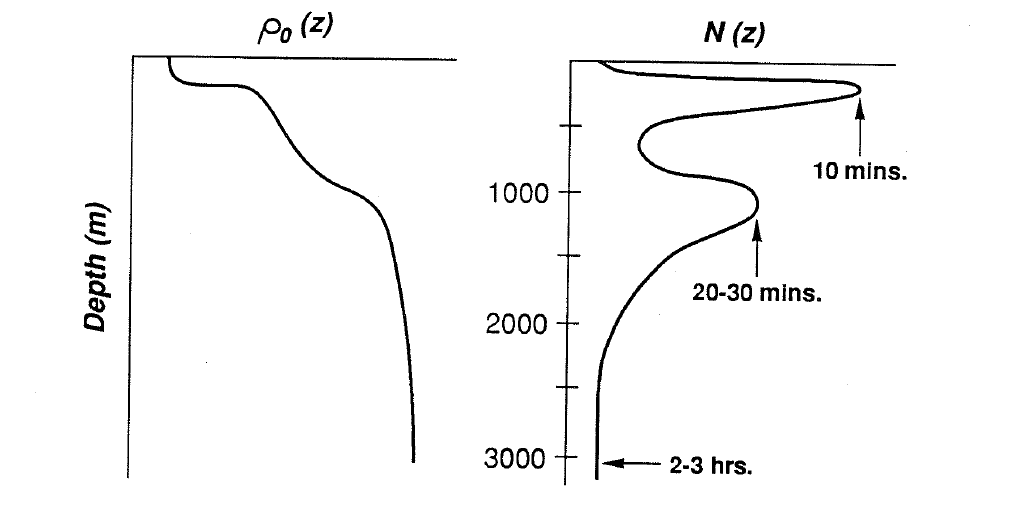
In most of the ocean $N^2>f^2$ although there are not many reliable values for the deepest parts of the ocean. With this sort of profile, we have $$R^2(z)=\frac{N^2(z)-\sigma^2}{\sigma^2-f^2}$$ and $R^2$ may be greater than or less than zero. We can examine the changes in the solution which result from this vertical dependence by looking for a wave solution like $$w=e^{-i\sigma t+ikx}\omega(z).$$ The waveguide internal wave problem becomes $$(\sigma^2-f^2)\omega_z-gk^2\omega=0\qquad\text{at }z=0$$ $$\omega_{zz}+k^2R^2(z)\omega=0$$

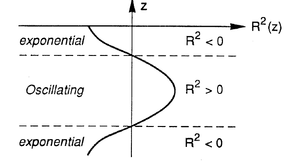
$$\omega=0\qquad\text{at }z=-D.$$ If $R^2(z)>0$, then the solution is trigonometric (travelling wave) because $\omega_{zz}/\omega<0$. If $R^2(z)<0$, then the solution is exponential (evanescent mode) because $\omega_{zz}/\omega>0$.

Suppose the $R^2(z)$ profile looks like

The system of equations is almost a Sturm–Liouville problem. We won’t go into the details of Sturm–Liouville theory because it can be found in many textbooks (and you should be familiar with it). We can summarize some relevant properties which will be useful for understanding the present problem. The usual Sturm–Liouville problem is $$(p\psi_z)_z+(q+\lambda r)\psi=0$$ $$a_{1,2}\psi_z+b_{1,2}\psi=0\qquad\text{at }z=0,-D$$ with $p,r>0$; $q<0$ or $q>0$. The parameters $p,q,r,a,b$ are all real. There is a singly infinite, denumerable set of eigenvalues $$\lambda_1\le\lambda_2\le\lambda_3\le\cdots\to\infty.$$ The eigenfunctions are orthogonal and can be orthonormalized as $$\int_{-D}^{0}\psi_i\psi_jr(z)\,dz=\delta_{ij}$$ where $\delta_{ij}$ is the Kronecker delta.

In terms of the Sturm–Liouville notation, we have $$\lambda=k^2,\qquad r=R^2(z),\qquad p=1,\qquad q=0.$$ Our present problem differs from the standard Sturm–Liouville problem in two ways. First, the eigenvalue $k^2$ appears in the boundary condition at $z=0$. Second, $R^2(z)$ may change sign in $-D<z<0$. Let’s look at each of these differences. When $R^2(z)$ changes sign in the definition interval, the generalized Sturm–Liouville theory demonstrates the existence of an infinite, denumerable set of eigenvalues which are real and have no lower bound to the sequence $$-\infty<\cdots<(k_2^e)^2<(k_1^e)^2<0<(k_1^w)^2<(k_2^w)^2<\cdots<+\infty$$ where the superscript $e$ represents an evanescent mode, and the superscript $w$ represents a travelling wave. The situation corresponds to

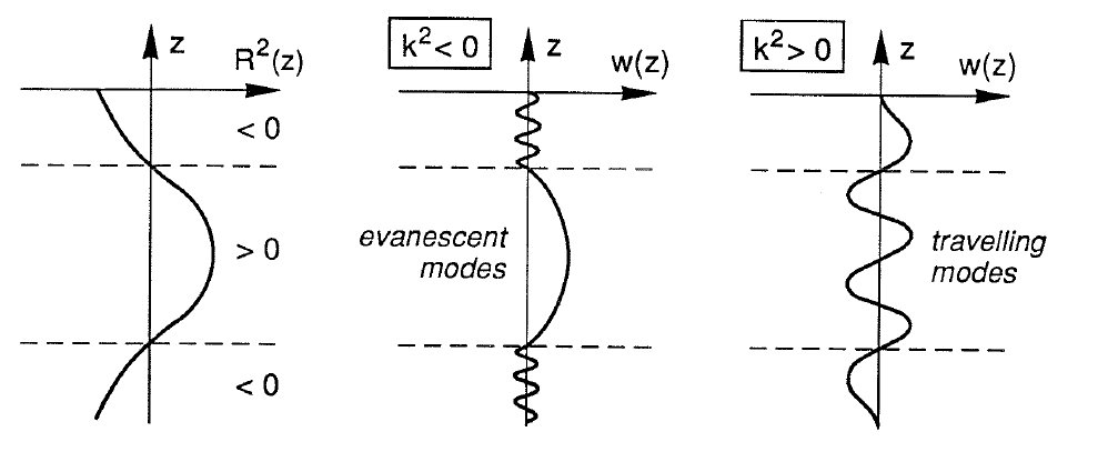
Thus, in this case, both evanescent and travelling modes are present simultaneously.

The effect of the appearance of $k^2$ in the surface boundary condition manifests itself as $$\int_{-D}^{0}\omega_i\omega_jR^2(z)\,dz =-\omega_i(0)\omega_j(0)g/(\sigma^2-f^2).$$

This says that the eigenfunctions $\omega_i$ are not orthogonal unless the surface boundary is the rigid lid, i.e. $\omega_i(0)=0$.

We could have solved the problem using the WKB approach in the case of slowly varying $N^2(z)$, but we don’t have time for that here. We can summarize the situation for $R^2(z)$ as follows. If $R^2(z)$ does not change sign in the water column, then all of the results found for the $N^2=\text{constant}$ case apply, with the only changes being in the details of the dispersion relation and in the vertical dependence of the velocity field. If $R^2(z)$ changes sign in the water column, then there is an infinite number of evanescent modes and travelling waves present simultaneously. If $\sigma^2>f^2$, there are also two travelling surface waves; if $\sigma^2<f^2$, there are two evanescent surface modes.